Page 71 - Read Online

Zhang et al. Intell Robot 2022;2(4):371­90 I http://dx.doi.org/10.20517/ir.2022.26 Page 377

The T-S fuzzy modelling approach is then employed to describe the time-varying car-following dynamics. We
use the classical sector nonlinearity method to derive the discrete-time T-S fuzzy model given in Equation (9):

Fuzzy rule ℛ : if 1 ( ) ∈ ℱ and 2 ( ) ∈ ℱ , then
1 2
( + 1) = ( + Δ ) ( ) + ( ) + ( + Δ ) ( ), (10)

where = 1, 2, · · · , , 1 ( ) = 1 and 2 ( ) = 1 2 are premise variables, ℱ is the fuzzy set, and , , Δ and
2
2
Δ are the system matrices defined in Equation (9), with 2 being replaced by min and max. We use ( ( ))

to denote the normalized membership function of ℱ , where ( ) = [ 1 ( ), 2 ( )] represents the premise

variable vector, ℱ = ℱ ℱ and ∑ ( ( )) = 1. For brevity, ( ( )) is denoted as . Considering the

1 2 =1
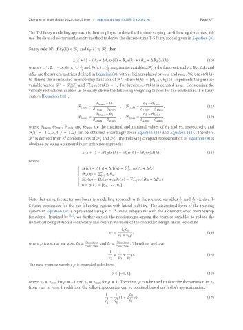
velocity restrictions enables us to easily derive the following weighting factors for the established T-S fuzzy
system [Equation (10)]:
1max − 1 1 − 1min
ℱ 1max = , ℱ 1min = , (11)
1max − 1min 1max − 1min
2max − 2 2 − 2min
ℱ 2max = , ℱ 2min = , (12)
2max − 2min 2max − 2min
where 1max, 2max, 1min and 2min are the maximal and minimal values of 1 and 2, respectively, and
ℱ ( = 1, 2, 3, 4, = 1, 2) can be obtained accordingly from Equation (11) and Equation (12). Therefore,

ℱ is derived from 2 combinations of ℱ and ℱ . The following compact representation of Equation (9) is

2
1 2
obtained by using a standard fuzzy inference approach:
( + 1) = ( ) ( ) + ℬ ( ) + ℬ ( ) ( ), (13)
where
∑
 ( ) = ( ) + Δ ( ) = ( + Δ )
 =1
 ∑

 ℬ ( ) =
=1
∑
 ℬ ( ) = ( ) + Δ ( ) = ( + Δ )
 =1


 = ( ) = [ 1 , · · · , ].
Note that using the sector nonlinearity modelling approach with the premise variables 1 and 1 yields a T-
2 2 2
S fuzzy expression for the car-following system with lateral stability. The discretized form of the tracking
system in Equation (9) is represented using = 2 linear subsystems with the aforementioned membership
2
functions. Inspired by [33] , we further exploit the relationships among the premise variables to reduce the
numerical computational complexity and conservativeness of the controller design. Here, we define
ˆ 0 ˆ 1
2 = , (14)
ˆ 1 + ˆ 0
where is a scalar variable, ˆ 0 = 2 min max and ˆ 1 = 2 min max . Therefore, we have
min + max min − max
1 1 1
= + . (15)
2 ˆ 0 ˆ 1
The new premise variable is bounded as follows:
∈ [−1, 1], (16)

where 2 = min for = −1 and 2 = max for = 1. Therefore, can be used to describe the variation in 2
from min to max. In addition, the following equation can be obtained based on Taylor’s approximation:

1 1 ˆ 0
' (1 + 2 ). (17)
2 ˆ 2 ˆ 1
2 0