Page 70 - Read Online

Page 376 Zhang et al. Intell Robot 2022;2(4):371­90 I http://dx.doi.org/10.20517/ir.2022.26

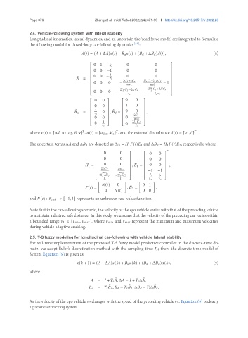
2.4. Vehicle­following system with lateral stability
Longitudinal kinematics, lateral dynamics, and an uncertain tire/road force model are integrated to formulate
the following model for closed-loop car-following dynamics [32] :

˜
˜
˜
˜
˜
¤ ( ) = ( + Δ ) ( ) + ( ) + ( + Δ ) ( ), (8)
 0 1 − 0 0 0 
 
 
 0 0 −1 0 0 
 1 
˜
=  0 0 − 0 0 0  

2 +2 2 −2
 0 0 0 − − 1 
 2 2 
 2 2 2 
 2 −2 2 +2 

 0 0 0 − − 
 2 
 0 0   0 0 
   
 0 0   1 0 
   
˜  1  ˜  0 0   ,
=  0  , = 
 0   2 
 0 0   0 
 1   2 
 0   0 2 
   

where ( ) = [Δ , Δ , 2 , , ] , ( ) = [ des , ] , and the external disturbance ( ) = [ 1 , ] .

˜
˜
˜
˜
˜
The uncertain terms Δ and Δ are denoted as Δ = 1 ( ) 1 and Δ = 1 ( ) 2, respectively, where
˜
˜
˜

 0 0   0 0 
   
 0 0   0 0 
   


˜  0 0   , 1 =  0 0  ,
˜
1 = 
 2Δ 2Δ   
   −1 −1 
2 2
   
2 Δ −
 −2 Δ   
   
[ ] [ ]
( ) 0 0 1
˜
( ) = , 2 = ,
0 ( ) 0 0
and ( ) : ≥0 → [−1, 1] represents an unknown real-value function.
Note that in the car-following scenario, the velocity of the ego vehicle varies with that of the preceding vehicle
to maintain a desired safe distance. In this study, we assume that the velocity of the preceding car varies within
a bounded range 1 ∈ [ min , max ], where min and max represent the minimum and maximum velocities
during vehicle adaptive cruising.
2.5. T­S fuzzy modeling for longitudinal car­following with vehicle lateral stability
For real-time implementation of the proposed T-S fuzzy model predictive controller in the discrete-time do-
main, we adopt Euler’s discretization method with the sampling time ; then, the discrete-time model of
System Equation (8) is given as
( + 1) = ( + Δ ) ( ) + ( ) + ( + Δ ) ( ), (9)
where
˜
˜
= + , Δ = + Δ ,
˜
˜
˜
= , = , Δ = Δ .
As the velocity of the ego vehicle 2 changes with the speed of the preceding vehicle 1, Equation (9) is clearly
a parameter-varying system.