Page 37 - Read Online

Sellers et al. Intell Robot 2022;2(4):333­54 I http://dx.doi.org/10.20517/ir.2022.21 Page 343

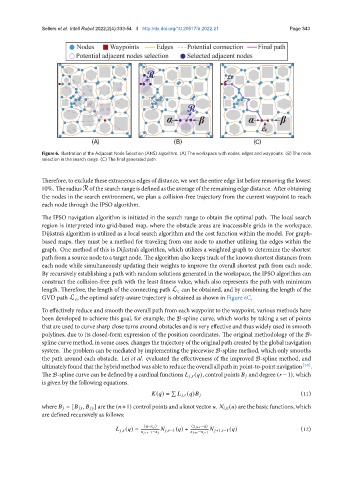
Figure 6. Illustration of the Adjacent Node Selection (ANS) algorithm. (A) The workspace with nodes, edges and waypoints. (B) The node
selection in the search range. (C) The final generated path.

Therefore, to exclude these extraneous edges of distance, we sort the entire edge list before removing the lowest
10%. The radius R of the search range is defined as the average of the remaining edge distance. After obtaining
the nodes in the search environment, we plan a collision-free trajectory from the current waypoint to reach
each node through the IPSO algorithm.

The IPSO navigation algorithm is initiated in the search range to obtain the optimal path. The local search
region is interpreted into grid-based map, where the obstacle areas are inaccessible grids in the workspace.
Dijkstra’s algorithm is utilized as a local search algorithm and the cost function within the model. For graph-
based maps, they must be a method for traveling from one node to another utilizing the edges within the
graph. One method of this is Dijkstra’s algorithm, which utilizes a weighted graph to determine the shortest
path from a source node to a target node. The algorithm also keeps track of the known shortest distances from
each node while simultaneously updating their weights to improve the overall shortest path from each node.
By recursively establishing a path with random solutions generated in the workspace, the IPSO algorithm can
construct the collision-free path with the least fitness value, which also represents the path with minimum
length. Therefore, the length of the connecting path L can be obtained, and by combining the length of the
GVD path L , the optimal safety-aware trajectory is obtained as shown in Figure 6C.
To effectively reduce and smooth the overall path from each waypoint to the waypoint, various methods have
been developed to achieve this goal, for example, the B-spline curve, which works by taking a set of points
that are used to curve sharp close turns around obstacles and is very effective and thus widely used in smooth
polylines, due to its closed-form expression of the position coordinates. The original methodology of the B-
spline curve method, in some cases, changes the trajectory of the original path created by the global navigation
system. The problem can be mediated by implementing the piecewise B-spline method, which only smooths
the path around each obstacle. Lei et al. evaluated the effectiveness of the improved B-spline method, and
ultimately found that the hybrid method was able to reduce the overall all path in point-to-point navigation [38] .
The B-spline curve can be defined by a cardinal functions , ( ), control points and degree ( −1), which
is given by the following equations.
∑
( ) = , ( ) (11)
where = [ , ] are the ( +1) control points and a knot vector . , ( ) are the basic functions, which
are defined recursively as follows:

( − ) ( + − )
, ( ) = , −1 ( ) + +1, −1 ( ) (12)
+ −1 − + − +1