Page 32 - Read Online

Page 338 Sellers et al. Intell Robot 2022;2(4):333­54 I http://dx.doi.org/10.20517/ir.2022.21

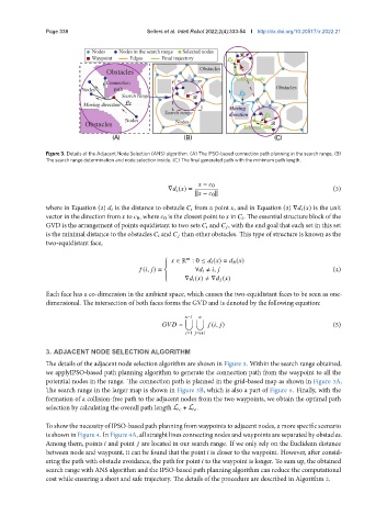
Figure 3. Details of the Adjacent Node Selection (ANS) algorithm. (A) The IPSO-based connection path planning in the search range. (B)
The search range determination and node selection inside. (C) The final generated path with the minimum path length.

− 0
∇ ( ) = (3)
k − 0 k
where in Equation (2) is the distance to obstacle from a point , and in Equation (3) ∇ ( ) is the unit
vector in the direction from to 0, where 0 is the closest point to in . The essential structure block of the
GVD is the arrangement of points equidistant to two sets and , with the end goal that each set in this set
is the minimal distance to the obstacles and than other obstacles. This type of structure is known as the
two-equidistant face,

 ∈ R : 0 ≤ ( ) = ℎ ( )


( , ) = ∀ ≠ , (4)

 ∇ ( ) ≠ ∇ ( )

Each face has a co-dimension in the ambient space, which causes the two-equidistant faces to be seen as one-
dimensional. The intersection of both faces forms the GVD and is denoted by the following equation:
−1
∪ ∪
= ( , ) (5)
=1 = +1

3. ADJACENT NODE SELECTION ALGORITHM
The details of the adjacent node selection algorithm are shown in Figure 3. Within the search range obtained,
we applyIPSO-based path planning algorithm to generate the connection path from the waypoint to all the
potential nodes in the range. The connection path is planned in the grid-based map as shown in Figure 3A.
The search range in the larger map is shown in Figure 3B, which is also a part of Figure 6. Finally, with the
formation of a collision-free path to the adjacent nodes from the two waypoints, we obtain the optimal path
selection by calculating the overall path length L + L .

To show the necessity of IPSO-based path planning from waypoints to adjacent nodes, a more specific scenario
is shown in Figure 4. In Figure 4A, all straight lines connecting nodes and waypoints are separated by obstacles.
Among them, points and point are located in our search range. If we only rely on the Euclidean distance
between node and waypoint, it can be found that the point is closer to the waypoint. However, after consid-
ering the path with obstacle avoidance, the path for point to the waypoint is longer. To sum up, the obtained
search range with ANS algorithm and the IPSO-based path planning algorithm can reduce the computational
cost while ensuring a short and safe trajectory. The details of the procedure are described in Algorithm 2.