Page 53 - Read Online

Page 146 Ortiz et al. Intell Robot 2021;1(2):131-50 I http://dx.doi.org/10.20517/ir.2021.09

Figure 11. The environment of the autonomous navigation.

8
6
9
10
4
2
y (m) 2 11 6
3
0 1
7
5
-2
4
8
-4 13
12
-6
-5 0 5 10 15 20
x (m)
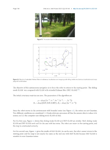
Figure 12. Results of extended Kalman filter simultaneous localization and mapping and sliding mode simultaneous localization and map-
ping with small noises.

The objective of this autonomous navigation is to force the robot to return to the starting point. The sliding
mode SLAM was compared with SLAM with extended Kalman filter (EKF-SLAM) [52] .

The initial covariance matrices are zero. The parameters of the algorithm are

−3 −3 −3 −4 −4
= ([1 , 1 , 4 , 2 , · · · , 2 ])
−4 −5
1 = ([0.05, 0.05, 0.005]), 2 = ([6 , 1 ])

Since the robot moves in the environment with bounded noise (see Figure 11), the noises are not Gaussian.
Two different conditions are considered: (1) Koala robot pre-processes off-line the sensors data to reduce 90%
noises; and (2) the computer uses sliding mode SLAM on-line.

For the first case, Figure 12 shows that sliding mode SLAM and EKF-SLAM are similar. Both sliding mode
SLAM and EKF-SLAM work well for the case with less noise. The robot can return to the starting point, and
the map is constructed correctly.

For the second case, Figure 13 gives the results of EKF-SLAM. As can be seen, the robot cannot return to the
starting point and the map is not exactly the same as the real one with EKF-SLAM because EKF-SLAM is
sensitive to non-Gaussian noises.