Page 49 - Read Online

Page 142 Ortiz et al. Intell Robot 2021;1(2):131-50 I http://dx.doi.org/10.20517/ir.2021.09

g(x ,x )
i j
100
x B SLAM
90 i
80
70 f*
60
y [m] 50
40
30
20
10
0
0 10 20 30 40 50 60 70 80 90 100
x [m]
Figure 3. Sliding mode simultaneous localization and mapping.

100 B f* x
obs T
B
90 SLAM
80
70
60
y [m] 50
40
30
x
S
20
10
0
0 10 20 30 40 50 60 70 80 90 100
x [m]
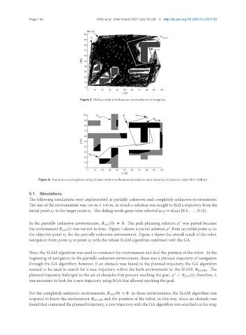
Figure 4. Autonomous navigation using sliding mode simultaneous localization and mapping and genetic algorithm method.

5.1. Simulations
The following simulations were implemented in partially unknown and completely unknown environments.
The size of the environments was 100 m × 100 m, in which a solution was sought to find a trajectory from the
initial point to the target point . The sliding mode gains were selected as = ([0.1, · · · , 0.1]).

In the partially unknown environments, (0) ≠ ∅. The path planning solution was partial because
∗
the environment ( ) was variant in time. Figure 3 shows a partial solution from an initial point to
∗
the objective point for the partially unknown environment. Figure 4 shows the overall result of the robot
navigation from point to point with the robust SLAM algorithm combined with the GA.

Here, the SLAM algorithm was used to construct the environment and find the position of the robot. At the
beginning of navigation in the partially unknown environment, there was a planned trajectory of navigation
through the GA algorithm; however, if an obstacle was found in the planned trajectory, the GA algorithm
needed to be used to search for a new trajectory within the built environment by the SLAM, . The
planned trajectory belonged to the set of obstacles that prevent reaching the goal, ⊂ ( ); therefore, it
∗
was necessary to look for a new trajectory using RGA that allowed reaching the goal.

For the completely unknown environments, (0) = ∅. In these environments, the SLAM algorithm was
required to know the environment and the position of the robot; in this way, when an obstacle was
found that contained the planned trajectory, a new trajectory with the GA algorithm was searched on the map