Page 41 - Read Online

Page 134 Ortiz et al. Intell Robot 2021;1(2):131-50 I http://dx.doi.org/10.20517/ir.2021.09

k u -
+ ˆ X k +1 X ˆ -
F (X ˆ + k ,u k ) k h (X ˆ - k )
+
k Z ˆ

- k Z
k e
+ +
k e
- +
X ˆ + +
k
K k e
k

K
k
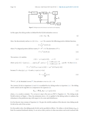
Figure 1. Sliding mode simultaneous localization and mapping.
In this paper, the sliding surface is defined by the SLAM estimation error as
(8)
( ) = x − ˆx

Here, the discontinuity surface is ( ) = [ 1 · · · ]. We consider the following positive definite function,
1
= ( ) ( ) (9)
2
where is diagonal positive definite matrix, = > 0. The derivative of is

¤ (10)
= ( ) ¤ ( )

The motion ( ) satisfies
¤ ( ) = − × [ ( )] , > 0 (11)
1 with ( ) > 0

where [ ( )] = [ ( 1 ) , . . . , ( )] , ( ) = , (0) = 0, then (10) is
−1 with ( ) < 0

¤
= ( ) {− × [ ( )]} = − ( ) [ ( )]
because = { } , > 0, and × ( ) = | |

· Õ
= − | | (12)
=1

Thus, ≤ 0. By Barbalat’s lemma [48] , the estimation error is ( ) → 0.
¤
The classical SLAM in Equations (4) and (5) is modified by the sliding surface in Equation (11). The sliding
mode control can be regarded as a compensator for Equation (4):

ˆ x +1 = F(ˆx ,u ) − × [ ( )] (13)

where is a positive constant. The correction step is the same as EKF in Equation (5). The sliding mode
SLAM is shown in Figure 1. Here, the estimation error, ( ), is applied to the sliding surface to enhance the
robustness in the prediction step with respect to the noise and disturbances.

It is the discrete-time version of Equation (6). We give the stability analysis of this discrete-time sliding mode
SLAM at the end of this section.

For the mobile robot, the sliding mode SLAM can be specified as follows. We define a critical distance min to
limit the maximal landmark density. It can reduce false positives in data association and avoid overload with