Page 43 - Read Online

Page 136 Ortiz et al. Intell Robot 2021;1(2):131-50 I http://dx.doi.org/10.20517/ir.2021.09

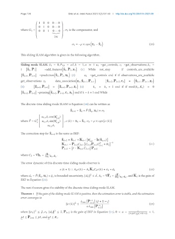
1 0 0 0 · · · 0
© ª
­ 0 1 0 0 · · · 0 ®
­ ® , is the compensator, and
®
where = ­ 0 0 1 0 · · · 0
­ ®
| {z }
­ ®
2
« ¬

= − × x − ˆx (20)
This sliding SLAM algorithm is given in the following algorithm.

Sliding mode SLAM. ˆ 1 = 0, 1|1 = , = 1, 1 1 =get_controls, 1 =get_observations; =

1 ˆ x 1 ,P 1 =add_features ˆx 1 ,P 1 ,z 1 (1) While not_stop if controls_are_available

=prediction ˆx ,P ,u (2) =get_controls end if if observations_are_available
ˆ x +1 ,P +1

get_observations data_association z , ˆx +1 ,P +1 ˆ x +2 ,P +2 ,c = ˆ x +1 ,P +1 ,z

(5) ˆ x +2 ,P +2 = ˆ x +2 ,P +2 ,z (1) = + 1 end if if mod( , ) = 0

ˆ x +2 ,P +2 =pruning ˆx +2 ,P +2 ,c ,a end if = + 1 end While
The discrete-time sliding mode SLAM in Equation (19) can be written as

ˆ
ˆ x +1 = ˆx + (ˆx ,u ) +

 , cos(x ) 
 , 


ˆ
where =  , sin(x )  , ( ) = x − ˆx , = × [ ( )]

 , 
 , 
 
The correction step for ˆx +2 is the same as EKF:

ˆ x +2 = ˆx +1 + K +1 z − h(ˆx )
+1 +1
−1
K +1 = P +2 +1 +1P +2 + 2 (21)
+1
P +2 = − K +1 +1 P +2
where = ∇h = h | .
x x =ˆx
The error dynamic of this discrete-time sliding mode observer is
( + 1) = ( ) − K ( ) + + (22)
F
¯
2
ˆ
where = (ˆx ,u ) + is bounded uncertainty, k k ≤ , = ∇F = x x =ˆx , and K is the gain of
|

EKF in Equation (21).
The next theorem gives the stability of the discrete-time sliding mode SLAM.
Theorem 1 If the gain of the sliding mode SLAM is positive, then the estimation error is stable, and the estimation
error converges to

max P −1 ( ¯ + ¯ ) + ¯
2 +1
k ( )k ≤ (23)
min P −1
+2
2
2

where k k ≤ ¯ , k k ≤ ¯, P +2 is the gain of EKF in Equation (21), 0 < = 1 < 1,

2

(1+ ¯ ¯ / )(1+ ¯ ¯+ )
≤ P +2 ≤ ¯ , and ≤ 1 .