Page 40 - Read Online

Ortiz et al. Intell Robot 2021;1(2):131-50 I http://dx.doi.org/10.20517/ir.2021.09 Page 133

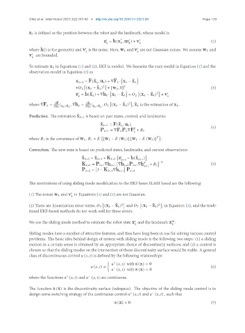
z is defined as the position between the robot and the landmark, whose model is

z = h(x ,m ) + v (2)

where h() is the geometry and v is the noise. Here, w and v are not Gaussian noises. We assume w and

v are bounded.

To estimate x in Equations (1) and (2), EKF is needed. We linearize the state model in Equation (1) and the
observation model in Equation (2) as

x +1 = F(ˆx ,u ) + ∇F · x − ˆx

2
+ 1 (x − ˆx ) + [w , 0] (3)

2
z = h(ˆx ) + ∇h · x − ˆx + 2 (x − ˆx ) + v

F h 2
where ∇F = | , ∇h = | , 1 (x − ˆx ) , ˆx is the estimation of x .
x x =ˆx x x =ˆx
Prediction. The estimation ˆx +1 is based on past states, control, and landmarks:
ˆ x +1 = F(ˆx ,u ) (4)

P +1 = ∇F P ∇F + 1

where 1 is the covariance of w , 1 = [w − (w )] [w − (w )] .
Correction. The new state is based on predicted states, landmarks, and current observations:

ˆ x +2 = ˆx +1 + K +1 z − h(ˆx )
+1 +1
−1
K +1 = P +1 ∇h +1 ∇h +1P +1 ∇h + 2 (5)
+1
P +2 = − K +1 ∇h +1 P +1
The motivations of using sliding mode modification to the EKF bases SLAM based are the following:

(1) The noises w and v in Equations (1) and (2) are not Gaussian.

(2) There are linearization error terms, 1 (x − ˆx ) and 2 (x − ˆx ) , in Equation (3), and the tradi-
2
2
tional EKF-based methods do not work well for these errors.

We use the sliding mode method to estimate the robot state x and the landmark x .

Sliding modes have a number of attractive features, and thus have long been in use for solving various control
problems. The basic idea behind design of system with sliding mode is the following two steps: (1) a sliding
motion in a certain sense is obtained by an appropriate choice of discontinuity surfaces; and (2) a control is
chosen so that the sliding modes on the intersection of those discontinuity surface would be stable. A general
class of discontinuous control ( , ) is defined by the following relationships:

( , ) with s (x) > 0
+
( , ) = (6)
( , ) with s (x) < 0
−
where the functions ( , ) and ( , ) are continuous.
+
−
The function s (x) is the discontinuity surface (subspace). The objective of the sliding mode control is to
design some switching strategy of the continuous control ( , ) and ( , ) , such that
−
+
s (x) = 0 (7)