Page 93 - Read Online

Page 81 Shu et al. Intell Robot 2024;4(1):74-86 I http://dx.doi.org/10.20517/ir.2024.05

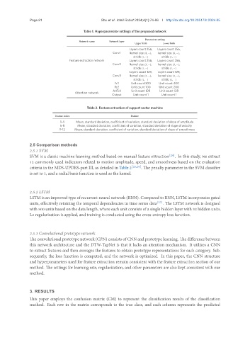
Table 1. Hyperparameter settings of the proposed network
Parameters setting
Network name Network layer
Upper limb Lower limb
Layers count 256, Layers count 256,
Conv1 kernel size (8, −), kernel size (8, −),
stride (1, −) stride (1, −)
Feature extraction network Layers count 256, Layers count 256,
Conv2 kernel size (5, −), kernel size (5, −),
stride (1, −) stride (1, −)
Layers count 128, Layers count 128,
Conv3 kernel size (3, −), kernel size (3, −),
stride (1, −) stride (1, −)
Fc1 Unit count 300 Unit count 400
Fc2 Unit count 100 Unit count 200
AttFc1 Unit count 128 Unit count 128
Attention network
Output Unit count 1 Unit count 1

Table 2. Feature extraction of support vector machine
Feature index Feature
1-4 Mean, standard deviation, coefficient of variation, standard deviation of slope of amplitude
5-8 Mean, standard deviation, coefficient of variation, standard deviation of slope of velocity
9-12 Mean, standard deviation, coefficient of variation, standard deviation of slope of smoothness

2.5 Comparison methods
2.5.1 SVM
SVM is a classic machine learning method based on manual feature extraction [24] . In this study, we extract
12 commonly used indicators related to motion amplitude, speed, and smoothness based on the evaluation
criteria in the MDS-UPDRS-part III, as detailed in Table 2 [25,26] . The penalty parameter in the SVM classifier
is set to 1, and a radial basis function is used as the kernel.

2.5.2 LSTM
LSTM is an improved type of recurrent neural network (RNN). Compared to RNN, LSTM incorporates gated
units, effectively retaining the temporal dependencies in time series data [27] . The LSTM network is designed
with 500 units based on the data length, where each unit consists of a single hidden layer with 32 hidden units.
L2 regularization is applied, and training is conducted using the cross-entropy loss function.

2.5.3 Convolutional prototype network
The convolutional prototype network (CPN) consists of CNN and prototype learning. The difference between
this network architecture and the DTW-TapNet is that it lacks an attention mechanism. It utilizes a CNN
to extract features and then averages the features to obtain prototype representations for each category. Sub-
sequently, the loss function is computed, and the network is optimized. In this paper, the CNN structure
and hyperparameters used for feature extraction remain consistent with the feature extraction section of our
method. The settings for learning rate, regularization, and other parameters are also kept consistent with our
method.

3. RESULTS
This paper employs the confusion matrix (CM) to represent the classification results of the classification
method. Each row in the matrix corresponds to the true class, and each column represents the predicted