Page 74 - Read Online

Yang et al. Intell Robot 2024;4(1):107-24 I http://dx.doi.org/10.20517/ir.2024.07 Page 113

the stepper motor has the same characteristics as the zero-order holder; it does not have any closed-loop en-
coder feedback for position control. Instead, it accepts a variation in the motor location as an input command
rather than the final motor location. In this paper, we used the variation in the motor location to tune the
supporting force of the support joint.

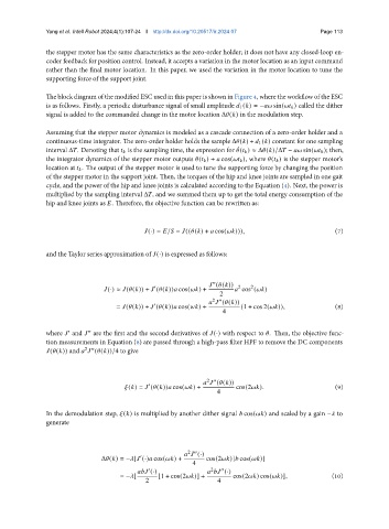
The block diagram of the modified ESC used in this paper is shown in Figure 4, where the workflow of the ESC
is as follows. Firstly, a periodic disturbance signal of small amplitude 1 ( ) = − sin( ) called the dither
signal is added to the commanded change in the motor location Δ ( ) in the modulation step.

Assuming that the stepper motor dynamics is modeled as a cascade connection of a zero-order holder and a
continuous-time integrator. The zero-order holder holds the sample Δ ( ) + 1 ( ) constant for one sampling
interval Δ . Denoting that is the sampling time, the expression for ( ) ≈ Δ ( )/Δ − sin( ); then,
¤
the integrator dynamics of the stepper motor outputs ( ) + cos( ), where ( ) is the stepper motor’s
location at . The output of the stepper motor is used to tune the supporting force by changing the position
of the stepper motor in the support joint. Then, the torques of the hip and knee joints are sampled in one gait
cycle, and the power of the hip and knee joints is calculated according to the Equation (4). Next, the power is
multiplied by the sampling interval Δ , and we summed them up to get the total energy consumption of the
hip and knee joints as . Therefore, the objective function can be rewritten as:

(·) = / = (( ( ) + cos( ))), (7)

and the Taylor series approximation of (·) is expressed as follows:

00
( ( ))
0 2 2
(·) ≈ ( ( )) + ( ( )) cos( ) + cos ( )
2
2 00
( ( ))
0 (1 + cos 2( )), (8)
= ( ( )) + ( ( )) cos( ) +
4
where and are the first and the second derivatives of (·) with respect to . Then, the objective func-
0
00
tion measurements in Equation (8) are passed through a high-pass filter HPF to remove the DC components
( ( )) and ( ( ))/4 to give
2 00

2 00
( ( ))
0 (9)
( ) = ( ( )) cos( ) + cos(2 ).
4
In the demodulation step, ( ) is multiplied by another dither signal cos( ) and scaled by a gain − to
generate

2 00
(·)
0
Δ ( ) = − [ (·) cos( ) + cos(2 )] cos( )]
4
0 2 00
(·) (·)
= − [ [1 + cos(2 )] + cos(2 ) cos( )], (10)
2 4