Page 53 - Read Online

Tong et al. Intell Robot 2024;4:125-45 I http://dx.doi.org/10.20517/ir.2024.08 Page 131

the iterative speed of target parameter convergence, thereby elevating identification accuracy. Atkeson et al.
employed a fifth-degree polynomial method as the excitation trajectory in joint space [36] . However, due to
the coupled relationship between joints in the joint space of the rehabilitation robot investigated in this study,
this method is not suitable. Swevers introduced, for the first time, an excitation trajectory model based on
Fourier series [37] . This trajectory possesses periodicity, smoothness, and strong robustness, making it widely
applicable in future research. Therefore, this paper adopts the Fourier series method for obtaining the excita-
tion trajectory, optimising the trajectory parameters based on the matrix condition number, and ultimately
obtaining a relatively ideal excitation trajectory. The signal-to-noise ratio of the data is improved by averag-
ing through multiple samples, enhancing data quality. The overdetermined equations used in the parameter
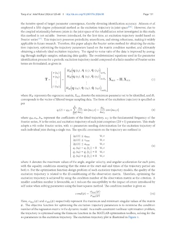
identification process for a periodic excitation trajectory model composed of a finite number of Fourier series
terms are formulated, as given in
. ..
 
 q ( 1 ) , q ( 1 ) , q ( 1 ) 
 ( 1 )   . .. × b 
   
 ( 2 )   q ( 2 ) , q ( 2 ) , q ( 2 ) 
    (7)

T =  . .  =  . × X min = H X min
 .   . 
   . 
   . .. 
 ( )   q ( ) , q ( ) , q ( ) 
 
 × 
where represents the regression matrix, denotes the minimum parameter set to be identified, and
corresponds to the vector of filtered torque sampling data. The form of the excitation trajectory is specified as
per

Õ

( ) = 0 + sin − cos (8)

=1
where 0 , , represent the coefficients of the fitted trajectory, is the fundamental frequency of the
Fourier series, is the order, and excitation trajectory of each joint comprises (2 +1) parameters. This study
adopts a 5th-order Fourier series, with 11 parameters needing determination for the excitation trajectory of
each individual joint during a single run. The specific constraints on the trajectory are outlined in
 ∀ ,
 | ( )| ≤ max


 ∀ ,
 | ¤ ( )| ≤ max



  ∀ ,
| ¥ ( )| ≤ max (9)

 ( 0 ) = = 0 ∀ ,



 ¤ ( 0 ) = ¤ = 0 ∀ ,



 ¥ ( 0 ) = ¥ = 0 ∀ ,

where A denotes the maximum values of the angle, angular velocity, and angular acceleration for each joint,
with the equality conditions ensuring that the states at the start and end times of the trajectory period are
both 0. For the optimisation function design problem of such excitation trajectory models, the quality of the
excitation trajectory is related to the ill-conditioning of the observation matrix. Therefore, optimising the
excitation trajectory is achieved by using the condition number of the observation matrix as the criterion. A
smaller condition number is favourable, as it reduces the susceptibility to the impact of errors introduced by
self-noise when solving parameters using the least squares method. The condition number is given as
max ( )
( ) = (10)
min ( )
Here, max ( ) and min ( ) respectively represent the maximum and minimum singular values of the matrix
. The objective function for optimising the excitation trajectory parameters is to minimise the condition
number of the regression matrix in the dynamic model. As a multi-constraint nonlinear optimisation problem,
the trajectory is optimised using the fmincon function in the MATLAB optimisation toolbox, solving for the
44 parameters in the excitation trajectory. The excitation trajectory plot is illustrated in Figure 3.