Page 71 - Read Online

Yang et al. Intell Robot 2024;4(4):406-21 I http://dx.doi.org/10.20517/ir.2024.24 Page 414

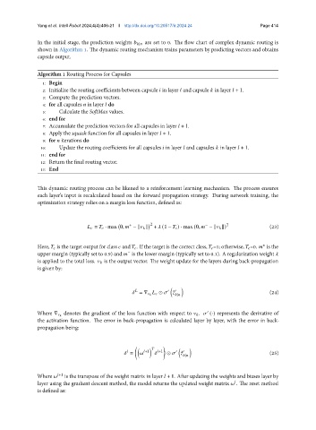
In the initial stage, the prediction weights | are set to 0. The flow chart of complex dynamic routing is
shown in Algorithm 1. The dynamic routing mechanism trains parameters by predicting vectors and obtains
capsule output.

Algorithm 1 Routing Process for Capsules
1: Begin
2: Initialize the routing coefficients between capsule in layer and capsule in layer + 1.
3: Compute the prediction vectors.
4: for all capsules in layer do
5: Calculate the SoftMax values.
6: end for
7: Accumulate the prediction vectors for all capsules in layer + 1.
8: Apply the squash function for all capsules in layer + 1.
9: for iterations do
10: Update the routing coefficients for all capsules in layer and capsules in layer + 1.
11: end for
12: Return the final routing vector.
13: End

This dynamic routing process can be likened to a reinforcement learning mechanism. The process ensures
each layer’s input is recalculated based on the forward propagation strategy. During network training, the
optimization strategy relies on a margin loss function, defined as:

2
+ − 2 (23)
= · max 0, − ∥ ∥ + (1 − ) · max (0, − ∥ ∥)

Here, is the target output for class and . If the target is the correct class, =1; otherwise, =0. is the
+
upper margin (typically set to 0.9) and is the lower margin (typically set to 0.1). A regularization weight
−
is applied to the total loss. is the output vector. The weight update for the layers during back-propagation
is given by:

′ ′ (24)
|
= ∇ ⊙ ˆ

denotes the gradient of the loss function with respect to . (·) represents the derivative of
′
Where ∇
the activation function. The error in back-propagation is calculated layer by layer, with the error in back-
propagation being:

′
= +1 +1 ⊙ ˆ ′ (25)
|
Where +1 is the transpose of the weight matrix in layer + 1. After updating the weights and biases layer by

layer using the gradient descent method, the model returns the updated weight matrix . The reset method
is defined as: