Page 67 - Read Online

Yang et al. Intell Robot 2024;4(4):406-21 I http://dx.doi.org/10.20517/ir.2024.24 Page 410

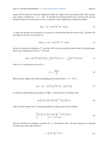
squares (WLS) method is commonly employed to adjust the weight of the measurement values. The measure-
ment residual is defined as = − ℎ( ). To quantify the deviation between the measured value and the
estimated value, the objective function is expressed as the weighted sum of squared residuals:

= ( − ℎ ( )) −1 ( − ℎ( )) (3)

To obtain the optimal state estimation, it is necessary to minimize the objective function Therefore, the
new objective function can be written as:

= ( − ℎ ( )) −1 ( − ℎ( )) (4)

Assume the initial state estimate is , such that ℎ( ) is linear around the initial estimate. By performing a
( )
Taylor series expansion of ℎ( ) at we obtain:
( )

1 1
2
′
ℎ( ) = ℎ (0) + (0) Δ + (0) (Δ ) + · · · + ( ) ( ) (Δ ) (5)
2 !
Where (·) is the Jacobian matrix of ℎ(·).

ℎ( )
(·) = (6)

Substituting the higher-order terms and applying the formula and let ˜ = − ℎ( ):
( )

= ˜ − ( ) Δ −1 ˜ − ( ) Δ (7)

To obtain the optimal objective function, set = 0 and solve for the estimate of Δˆ:

Δ

(−1)
−1
−1

Δˆ= ( ) ( ) ( ) (8)
˜
Thus, the state estimate vector is iteratively updated according to the iterative formula:

 (−1)
 −1 −1

  Δˆ= ( ) ( ) ( )
˜
(9)
 ( +1) ( )

 = + Δˆ

When Δˆ satisfies the convergence condition Δˆ ≤ , the iteration stops. The state estimate Δˆ is obtained.

The final value of the state estimate is:
−1

−1
−1
ˆ = (10)