Page 9 - Read Online

Sathyan et al. Complex Eng Syst 2022;2:18 I http://dx.doi.org/10.20517/ces.2022.41 Page 5 of 12

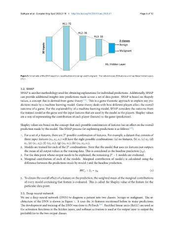
Figure 1. Schematic of the DNN used for classification into benign and malignant. The network uses 30 features and has three hidden layers
(HL).

3.2. SHAP
SHAP is another methodology used for obtaining explanations for individual predictions. Additionally, SHAP
can provide additional insights into predictions made across a set of data points. SHAP is based on Shapely
values, a concept that is derived from game theory [16] . This is a game theoretic approach to explain any pre-
dictions made by a machine learning model. Game theory deals with how different players affect the overall
outcome of a game. For the explainability of a machine learning model, SHAP considers the outcome from
the trained model as the game and the input features that are used by the model as the players. Shapley values
are a way of representing the contribution of each player (feature) to the game (prediction).

Shapley values are based on the concept that each possible combination of features has an effect on the overall
prediction made by the model. The SHAP process for explaining predictions is as follows [27] :

1. For a set of features, there are 2 possible combination of features. For example, a dataset that consists of

three input features ( 1 , 2 , 3) will have the eight possible combinations: (a) no features, (b) 1 (c) 2, (d)
3, (e) ( 1 , 2 ), (f) ( 2 , 3 ), (g) ( 1 , 3 ), (h) ( 1 , 2 , 3 ).

2. Models are trained for each of the 2 combinations. Note that the model that uses no features just outputs
the mean of all output values in the training data. This is considered as the baseline prediction ( ).

3. For the data point whose output needs to be explained, the remaining 2 − 1 models are evaluated.
4. Marginal contribution of each of the models. Marginal contribution of model-j is calculated using the
difference between the predictions made by model-j and the baseline prediction.

(1)
= ˜ −
5. To obtain the overall effect of a feature on the prediction, the weighted mean of the marginal contributions
of every model containing that feature is evaluated. This is called the Shapley value of the feature for the
particular data point.

3.3. Deep neural network
We use a deep neural network (DNN) to diagnose a patient into two classes: benign or malignant. The ar-
chitecture of the DNN is shown in Figure 1. It uses the 30 features mentioned before to make predictions.
The development and training of the DNN was done in PyTorch [28] . Rectified linear units (ReLU) are used as
the activation functions in the hidden layers, and softmax activation is used at the output layer to output the
probabilities to the two output classes.