Page 91 - Read Online

Page 8 of 23 Yu et al. Carbon Footprints 2025, 4, 17 https://dx.doi.org/10.20517/cf.2025.12

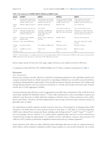
Table 2. The comparison of COPERT, EMFAC, MOBILE and HBEFA models
Model COPERT EMFAC MOBILE HBEFA
Input Average speed, vehicle fleet Average speed, vehicle fleet Average speed, vehicle fleet Traffic situation, vehicle fleet
composition, vehicle activity, composition, vehicle activity, composition, vehicle activity, composition, vehicle activity,
weather conditions, etc. weather conditions, etc. weather conditions, etc. gradient, weather conditions, etc.
Spatial National, regional, local, link Regional, project level National, local City, project level
scale
Time scale Year, month, week, day, hour Year, season Year, season, month, day Year, month, week, day, hour
Vehicle Passenger cars, light-duty, Passenger cars, light-duty, Passenger cars, motorcycles, Passenger cars, light commercial
type heavy-duty, urban buses & heavy-duty, motorcycles, light- and heavy-duty trucks vehicles, heavy-duty trucks, urban
coaches, motorcycles medium-duty, buses, buses & coaches, motorcycles
motorcycle
Energy Gasoline, diesel, liquefied Gasoline, diesel, natural gas, Gasoline, diesel Gasoline, diesel, electricity
type petroleum gas electricity
Road type Urban, rural and highway / Highway Motorway, rural, urban, overall
average
Driving European countries FTP, California Unified Cycle Different counties European countries
cycle
Version COPERT 5.8.1, 2024 EMFAC 2021 MOBILE 6.2, 2004 HBEFA 4.2, 2022
Reference [33] [34] [35] [36]

COPERT: Computer program to calculate emissions from road transportation; EMFAC: emission factor; MOBILE: mobile source emissions factor;
HBEFA: handbook emission factors for road transport; FTP: federal test procedure.

power, engine speed, air/fuel ratio, fuel usage, engine emissions, and catalyst conversion efficiency.

A comparison of the MOVES, IVE, CMEM, PHEM, and VT-Micro models is summarized in Table 3.

Discussion
Data requirements
Microscopic emission models, which are suitable for estimating emissions at the individual vehicle level,
compute emissions based on vehicle trajectories or operating conditions at a second-by-second resolution,
resulting in substantial data requirements. These models incorporate dynamic parameters that continuously
change during operation, such as acceleration and speed. In contrast, macroscopic and mesoscopic emission
models rely on traffic aggregated variables.

Local governments typically have access to aggregated road traffic data, summarized at the traffic flow level
rather than classified by individual vehicle . Urban traffic infrastructure, such as surveillance cameras and
[9]
inductive loop detectors, is widely deployed, making it relatively easy to obtain parameters such as flow,
speed, and density. Therefore, the data requirements of macroscopic and mesoscopic emission models are
generally easier to satisfy.

For instantaneous vehicle emission models, trajectory data are a critical input for evaluating urban traffic
emissions. Currently, there are three primary sources of such data: (1) GPS data or on-board diagnostics
[46]
[49]
[45]
(OBD) data collected from commercial fleets, including ride-hailing services , taxis , buses [47,48] , trucks ,
[50]
and increasingly, electric vehicles ; (2) mobile phone signaling data and user location information
obtained from navigation applications; (3) roadside sensors, surveillance cameras, and electronic toll
collection (ETC) systems, particularly at signalized intersections and key roadway segments .
[51]
Sparse trajectory data, which are often collected at intervals longer than one second, are common; however,
most vehicle carbon emission estimation models require inputs at a one-second resolution. As a result,