Page 96 - Read Online

Page 12 of 23 Yu et al. Carbon Footprints 2025, 4, 17 https://dx.doi.org/10.20517/cf.2025.12

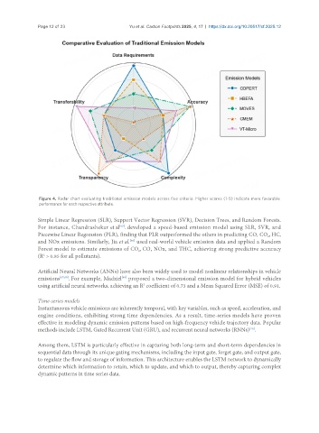
Figure 4. Radar chart evaluating traditional emission models across five criteria. Higher scores (1-5) indicate more favorable
performance for each respective attribute.

Simple Linear Regression (SLR), Support Vector Regression (SVR), Decision Trees, and Random Forests.
[65]
For instance, Chandrashekar et al . developed a speed-based emission model using SLR, SVR, and
Piecewise Linear Regression (PLR), finding that PLR outperformed the others in predicting CO, CO , HC,
2
and NOx emissions. Similarly, Jia et al. used real-world vehicle emission data and applied a Random
[66]
Forest model to estimate emissions of CO , CO, NOx, and THC, achieving strong predictive accuracy
2
(R > 0.85 for all pollutants).
2
Artificial Neural Networks (ANNs) have also been widely used to model nonlinear relationships in vehicle
emissions [67,68] . For example, Madziel proposed a two-dimensional emission model for hybrid vehicles
[69]
using artificial neural networks, achieving an R coefficient of 0.73 and a Mean Squared Error (MSE) of 0.91.
2
Time-series models
Instantaneous vehicle emissions are inherently temporal, with key variables, such as speed, acceleration, and
engine conditions, exhibiting strong time dependencies. As a result, time-series models have proven
effective in modeling dynamic emission patterns based on high-frequency vehicle trajectory data. Popular
[70]
methods include LSTM, Gated Recurrent Unit (GRU), and recurrent neural networks (RNNs) .

Among them, LSTM is particularly effective in capturing both long-term and short-term dependencies in
sequential data through its unique gating mechanisms, including the input gate, forget gate, and output gate,
to regulate the flow and storage of information. This architecture enables the LSTM network to dynamically
determine which information to retain, which to update, and which to output, thereby capturing complex
dynamic patterns in time series data.