Page 202 - Read Online

Wang et al. J. Mater. Inf. 2026, 6, 16 Page 5 of 25

regression, can accommodate non-overlapping MF datasets in which HF and LF data are observed at
different inputs . When domain knowledge suggests a credible approximation form for F, parametric MF
[64]
models are parsimonious, fast, and robust, providing a principled mechanism to prioritize HF data while still
leveraging LF samples to capture global trends.

In practice, parametric MF models are most effective in applications where domain expertise provides
guidance for a plausible functional form. For example, in hypersonic vehicle surface pressure modeling, MF
linear regression improved predictive accuracy by up to 12% compared to SF regression, even with as few as
3-10 HF samples . In materials science, heteroscedastic Gaussian process regression (HGPR) has been
[64]
applied to porous two-phase microstructures generated by finite element simulations. In this setting,
input-dependent noise captures inherently noisy regimes, linking geometric descriptors (ellipse axes,
porosity, spacing) to effective stress in representative volume element (RVE) (60%-40% split for training and
validation sets) . This study illustrates that heteroscedasticity in materials datasets, traditionally regarded as
[65]
a nuisance, can instead be leveraged as an informative signal to guide design and optimization.

These advantages, however, come with trade-offs. Parametric MF models often suffer from limited
representational capacity: linear or polynomial structures may be inadequate for highly nonlinear,
high-dimensional behaviors. They can also degrade when LF data introduce systematic bias or when fidelity
relationships deviate significantly from simple mappings. Furthermore, mis-specified fidelity-dependent
variances can undermine the intended emphasis on HF data. Such issues can be mitigated by re-estimating
variance terms via maximum likelihood or by extending the framework to include fidelity-specific offsets
and scaling factors .
[46]

From a practical standpoint, for parametric MF models, a key design choice is the selection of the functional
form. A practical strategy is to start from the simplest model justified by physical insight and progressively
increase complexity as needed. Candidate models can be evaluated using cross-validation, and the model
that exhibits the best generalization performance is selected.

Direct machine learning with fidelity features
A second strategy for MF learning is to directly encode fidelity information as an input feature to a unified
model. Rather than building separate models at each fidelity or linking them hierarchically, all data are
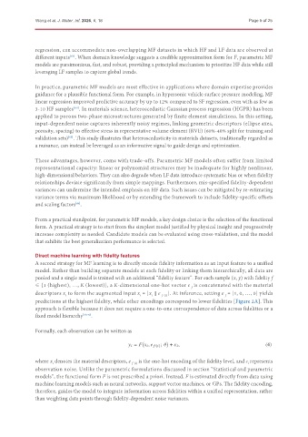
pooled and a single model is trained with an additional “fidelity feature”. For each sample (x, y) with fidelity f
∈ {1 (highest), …, K (lowest)}, a K-dimensional one-hot vector e is concatenated with the material
f
descriptors x to form the augmented input x = [x ǀǀ e ]. At inference, setting e = [1, 0, …, 0] yields
i
f (i)
f
i
i
predictions at the highest fidelity, while other encodings correspond to lower fidelities [Figure 2A]. This
approach is flexible because it does not require a one-to-one correspondence of data across fidelities or a
fixed model hierarchy [39,40] .
Formally, each observation can be written as

H 8 = G 8 , 4 5 (8) ; \ + Y 8 , (4)

where x denotes the material descriptors, e is the one-hot encoding of the fidelity level, and ε represents
i
f (i)
i
observation noise. Unlike the parametric formulations discussed in section “Statistical and parametric
models”, the functional form F is not prescribed a priori. Instead, F is estimated directly from data using
machine learning models such as neural networks, support vector machines, or GPs. The fidelity encoding,
therefore, guides the model to integrate information across fidelities within a unified representation, rather
than weighting data points through fidelity-dependent noise variances.