Page 11 - Read Online

Li et al. J Mater Inf 2024;4:27 https://dx.doi.org/10.20517/jmi.2024.44 Page 5 of 20

Finally, the selected design scheme undergoes validation through the CALPHAD and experimental
methods. If the new RAFM steel meets all design criteria, the process is complete. If not, the testing data are
added to the training dataset for the next iteration.

Data preparation
[32]
The dataset used in this study regarding the tensile properties of RAFM steels was from our former work .
For the microstructural dataset, it was collected from phase diagrams calculated by the Thermo-Calc
software with the TCFE10 database . Firstly, compositions and heat treatment parameters of RAFM steels
[33]
were collected from literature, and used as inputs for CALPHAD predictions. To ensure low activation and
reflect the typical compositions of RAFM steels, the following alloying elements were chosen: C, Cr, W, Si,
Mn, V, Ta, Ti, and N. The heat treatment parameters (NT; Nt: normalizing time; TT; Tt: tempering time)
were chosen based on commonly reported preparation conditions of RAFM steels, ensuring the
representativeness and reliability of the data. Secondly, CALPHAD step diagrams were digitized to obtain
the microstructural data for δ-ferrite, coarsening phases (i.e., Laves and Z-phase), V , and V M23C6 under
MX
different heat treatment parameters. Finally, the microstructural dataset included 209 samples with δ-ferrite
and 202 samples without (named Data-I); 76 samples with coarsening phases and 144 samples without
(named Data-II); 219 samples for V (named Data-III); 219 samples for V M23C6 (named Data-IV). The data
MX
distribution of the microstructural dataset is provided in Supplementary Figure 1. To reduce dimensional
differences and improve calculation accuracy, it was necessary to normalize the collected datasets to [0, 1].

ML algorithms
In this study, various ML algorithms were chosen to build prediction models, including decision tree,
random forest, support vector machine, gradient boosting, k-nearest neighbor, and artificial neural network.
The unique characteristics of each algorithm are outlined in the Supplementary Section 2. The decision tree
classifier (DTC), random forest classifier (RFC), support vector classifier (SVC), gradient boosting classifier
(GBC), k-nearest neighbor classifier (KNC), and artificial neural network classifier (ANNC) were used to
build the classification models. The effectiveness of these classification models was assessed based on their
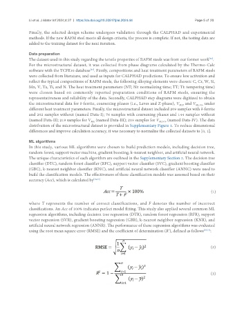
accuracy (Acc), which is calculated by [34,35]

(1)

where T represents the number of correct classifications, and F denotes the number of incorrect
classifications. An Acc of 100% indicates perfect model fitting. This study also applied several common ML
regression algorithms, including decision tree regression (DTR), random forest regression (RFR), support
vector regression (SVR), gradient boosting regression (GBR), k-nearest neighbor regression (KNR), and
artificial neural network regression (ANNR). The performance of these regression algorithms was evaluated
using the root mean square error (RMSE) and the coefficient of determination (R ), defined as follows [36,37] :
2

(2)

(3)