Page 70 - Read Online

Page 10 of 15 Hu et al. J Mater Inf 2023;3:1 I http://dx.doi.org/10.20517/jmi.2022.28

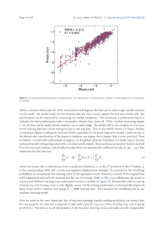
RMSE= 0.212
2 2
R = 0.892

3

ediction 4

r
P
5

6

7
5 4 3 2
Measured

Figure 6. Comparison of the machine learning predicted with the simulation measurements. A linear fit (red dashed line) is included for
illustration.

will be a variance-bias trade-off. With small polynomial degrees, the bias can be rather high, but the variance
can be small. The model under-fits the training data and thus cannot capture the test data trends well. The
performance can be improved by increasing the model complexity. The minimum at polynomial degree 6
indicates the best performance with a reasonable variance-bias trade-off. With a further increasing degree
(> 6), the bias can be small, but the variance can be rather high. The model will be too complex so as to over-
fit the training data but cannot well generalize to the test data. That is why RMSE shows a V-shape. Further
increasing to degree 8 will greatly increase RMSE, especially for the linear regression model. Given the size of
the dataset and consideration of the degree of freedom, any degree that is higher than 8 is not practical. Thus,
we believe a model with polynomials at degree 6 is the global optimum.Therefore, we would expect that the
optimizedmodelisRidgeregressionwithasix-degreepolynomial. Therearehencearound210featuresderived
from the four basic features. Specifically, this algorithm is to estimate the coefficient set { 0 , 1 , 2 , ..., } that
minimizes the loss function

∑ ∑ ∑
2
2
( − 0 − ) + , (5)

=1 =1 =1
th th
where the dataset has observations with predictors (features), is the predictor of the feature,
is the corresponding label, and is the non-negative regularization strength. To account for the overfitting
probability, we characterize the learning curve of the optimized model. Basically, a subset of the original data
will be generated internally for training and the rest for testing. With 10-fold cross-validations, the model is
trained with different training sizes, and its performance is plotted in Figure 5B. Remarkably, with increasing
training size, the training score is only slightly worse, but the testing performance is dramatically improved.
Both scores tend to saturate and merge at ∼ 3000 training data. This excludes the overfitting risk in our
machine-learning model.

Now we come to the most important step of machine learning, namely making predictions on unseen data.
For our purpose, we leave out a subgroup of data with a specific / before training (e.g., out-of-group
prediction). This aims to avoid interpolation in the machine learning model and make sure the independent