Page 69 - Read Online

Hu et al. J Mater Inf 2023;3:1 I http://dx.doi.org/10.20517/jmi.2022.28 Page 9 of 15
A B

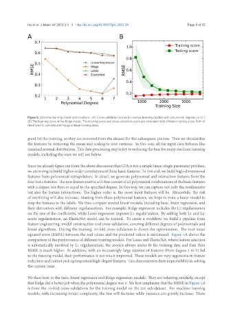
Figure 5. Machine learning model optimizations. (A) Cross-validation scores for various learning models with polynomial degrees up to 7.
(B) The learning curve of the Ridge model. The training score and cross-validation score are compared with different training sizes. Both of
them tend to saturate and merge at large training sizes.

good for the training, so they are removed from the dataset for the subsequent process. Then we standardize
the features by removing the mean and scaling to unit variance. In this way, all the input data behaves like
standard normal distribution. This data processing step is key to reducing the bias for many machine learning
models, including the ones we will use below.

Sincewe already figure out from theabove discussion that GFA is nota simple linear single parameter problem,
we are trying to build higher-order correlations of these basic features. To this end, we build high-dimensional
features from polynomial extrapolation. In detail, we generate polynomial and interaction features from the
fourbasicfeatures. Thenewfeaturematrixwillthusconsistofallpolynomialcombinationsofthebasicfeatures
with a degree less than or equal to the specified degree. In this way, we can capture not only the nonlinearity
but also the feature interactions. The higher order is, the more input features will be. Meanwhile, the risk
of overfitting will also increase. Starting from these polynomial features, we hope to train a linear model to
map the features to the labels. We thus compare several linear models, including basic linear regression, and
their derivatives with different regularizations. For example, Ridge regression includes the L2 regularization
on the size of the coefficients, while Lasso regression imposes L1 regularization. By adding both L1 and L2-
norm regularization, an ElasticNet model can be trained. To create a workflow, we build a pipeline from
feature engineering, model construction and cross validation, covering different degrees of polynomials and
linear algorithms. During the training, 10-fold cross validation is chosen for optimization. The root mean
squared error (RMSE) between the real values and the predicted values is minimized. Figure 5A shows the
comparison of the performance of different training models. For Lasso and ElasticNet, where feature selection
is automatically involved by L1 regularization, the models always under-fit the training data and thus their
RMSE is much higher. In addition, with an increasingly large number of features (from degree 1 to 7) fed
to the training model, their performance is not much improved. These models are very aggressive in feature
reductionandcannotpickupimportanthigh-degreefeatures. Thisdemonstratestheirimprobabilityinsolving
the current issue.

We then turn to the basic linear regression and Ridge regression models. They are behaving similarly, except
that Ridge did a better job when the polynomial degree was 6. We first emphasize that the RMSE in Figure 5A
is from the 10-fold cross-validations for the training model on the test sub-dataset. For machine learning
models, with increasing model complexity, the bias will decrease while variance can greatly increase. There