Page 19 - Read Online

Lei et al. Intell Robot 2022;2(4):313­32 I http://dx.doi.org/10.20517/ir.2022.18 Page 325

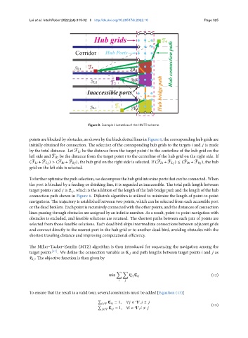
Figure 8. Example illustration of the HMTR scheme.

points are blocked by obstacles, as shown by the black dotted lines in Figure 8, the corresponding hub grids are
initially obtained for connection. The selection of the corresponding hub grids to the targets and is made
by the total distance. Let F be the distance from the target point to the centerline of the hub grid on the
left side and F be the distance from the target point to the centerline of the hub grid on the right side. If
(F + F ) > (F + F ), the hub grid on the right side is selected. If (F + F ) ≤ (F + F ), the hub
grid on the left side is selected.

Tofurtheroptimizethepathselection,wedecomposethehubgridintonineportsthatcanbeconnected. When
the port is blocked by a feeding or drinking line, it is regarded as inaccessible. The total path length between
target points and is , which is the addition of the length of the hub bridge path and the length of the hub
connection path shown in Figure 8. Dijkstra’s algorithm is utilized to minimize the length of point-to-point
navigations. The trajectory is established between two points, which can be selected from each accessible port
or the dead broilers. Each point is recursively connected with the other points, and the distances of connection
lines passing through obstacles are assigned by an infinite number. As a result, point-to-point navigation with
obstacles is excluded, and feasible solutions are retained. The shortest paths between each pair of points are
selected from those feasible solutions. Each dead bird skips intermediate connections between adjacent grids
and connect directly to the nearest port in the hub grid or to another dead bird, avoiding obstacles with the
shortest traveling distance and improving computational efficiency.

The Miller–Tucker–Zemlin (MTZ) algorithm is then introduced for sequencing the navigation among the
target points [37] . We define the connection variable as ℭ and path lengths between target points and as
. The objective function is then given by

∑ ∑
min ℭ (12)

To ensure that the result is a valid tour, several constraints must be added [Equation (13)]
∑
ℭ = 1, ∀ ∈ V, ≠
∈V (13)
∑
ℭ = 1, ∀ ∈ V, ≠
∈V