Page 8 - Read Online

Wu. Intell Robot 2021;1(2):99-115 I http://dx.doi.org/10.20517/ir.2021.11 Page 101

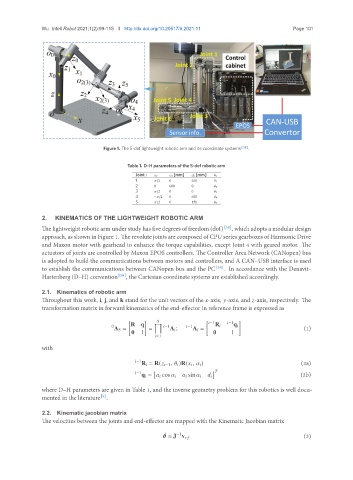
Figure 1. The 5-dof lightweight robotic arm and its coordinate systems [38] .

Table 1. D–H parameters of the 5-dof robotic arm
Joint [mm] [mm]
1 /2 0 250 1
2 0 600 0 2
3 /2 0 0 3
4 − /2 0 600 4
5 /2 0 150 5

2. KINEMATICS OF THE LIGHTWEIGHT ROBOTIC ARM
The lightweight robotic arm under study has five degrees of freedom (dof) [38] , which adopts a modular design
approach, as shown in Figure 1. The revolute joints are composed of CPU series gearboxes of Harmonic Drive
and Maxon motor with gearhead to enhance the torque capabilities, except Joint 4 with geared motor. The
actuators of joints are controlled by Maxon EPOS controllers. The Controller Area Network (CANopen) bus
is adopted to build the communications between motors and controllers, and A CAN–USB interface is used
to establish the communications between CANopen bus and the PC [38] . In accordance with the Denavit–
Hartenberg (D–H) convention [39] , the Cartesian coordinate systems are established accordingly.

2.1. Kinematics of robotic arm
Throughout this work, i, j, and k stand for the unit vectors of the -axis, -axis, and -axis, respectively. The
transformation matrix in forward kinematics of the end-effector in reference frame is expressed as

[ ] 5 [ −1 −1 ]
R q ∏
0 −1 −1 R q
A 5 = = A ; A = (1)
0 1 0 1
=1
with

−1 (2a)
R = R( −1 , )R( , )
−1 [ ] (2b)
q = cos sin
where D–H parameters are given in Table 1, and the inverse geometry problem for this robotics is well docu-
[8]
mented in the literature .
2.2. Kinematic jacobian matrix
The velocities between the joints and end-effector are mapped with the Kinematic Jacobian matrix

¤ −1 (3)
= J v