Page 14 - Read Online

Wu. Intell Robot 2021;1(2):99-115 I http://dx.doi.org/10.20517/ir.2021.11 Page 107

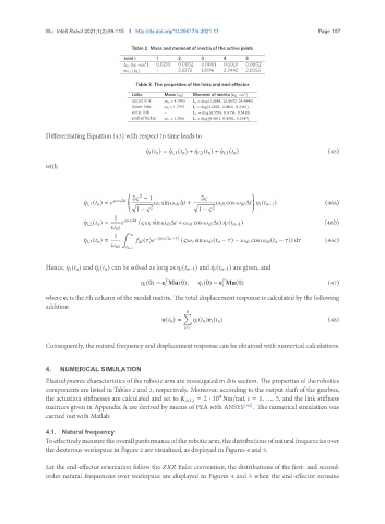
Table 2. Mass and moment of inertia of the active joints
Joint i 1 2 3 4 5
2 0.0210 0.0002 0.0001 0.0001 0.0002
, [kg · mm ]
, [kg] − 2.2272 1.8196 2.2442 2.0053
Table 3. The properties of the links and end-effector
Links Mass [kg] Moment of inerita [kg · cm ]
2
upper link = 4.7995 I = diag[1.1884, 25.0670, 24.4940]
lower link = 1.7795 I = diag[4.0802, 4.0861, 0.2345]
wrist link − I = diag[0.5556, 0.9154, 0.6119]
end-effector = 1.2961 I = diag[0.4563, 0.4382, 0.2347]
Differentiating Equation (43) with respect to time leads to

¤ ( ) = ¤ ,1 ( ) + ¤ ,2 ( ) + ¤ ,3 ( ) (45)
with

( )
2
2 − 1 2
¤ ,1 ( ) = Δ √ sin Δ + √ cos Δ ( −1 ) (46a)
1 − 2 1 − 2
1 Δ
¤ ,2 ( ) = ( sin Δ + cos Δ ) ¤ ( −1 ) (46b)

∫
1
¤ ,3 ( ) = ( ) − ( − ) ( sin ( − ) − cos ( − )) d (46c)

−1
Hence, ( ) and ¤ ( ) can be solved as long as ( −1 ) and ¤ ( −1 ) are given, and

(0) = e Mu(0); ¤ (0) = e M¤ u(0) (47)

where e is the th column of the modal matrix. The total displacement response is calculated by the following
addition
6
∑
u( ) = ( )e ( ) (48)
=1
Consequently, the natural frequency and displacement response can be obtained with numerical calculations.

4. NUMERICAL SIMULATION

Elastodynamic characteristics of the robotic arm are investigated in this section. The properties of the robotics
components are listed in Tables 2 and 3, respectively. Moreover, according to the output shaft of the gearbox,
the actuation stiffnesses are calculated and set to , = 2 · 10 Nm/rad, = 1, ..., 5, and the link stiffness
4
matrices given in Appendix A are derived by means of FEA with ANSYS [45] . The numerical simulation was
carried out with Matlab.

4.1. Natural frequency
To effectively measure the overall performance of the robotic arm, the distributions of natural frequencies over
the dexterous workspace in Figure 2 are visualized, as displayed in Figures 4 and 5.

Let the end-effector orientation follow the Euler convention; the distributions of the first- and second-
order natural frequencies over workspace are displayed in Figures 4 and 5 when the end-effector remains