Page 38 - Read Online

Bao et al. Complex Eng Syst 2022;2:16 I http://dx.doi.org/10.20517/ces.2022.30 Page 7 of 10

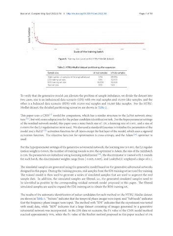
Figure 5. Training loss curve on the HTRU-Medlat dataset.

Table 2. HTRU-Medlat dataset partitioning after expansion

Sample size of real samples of fake samples
Total number of samples in the original dataset 1,196 89,996
IDS training set size 696 10,000
BDS training set size 10,000 10,000
Test set size 500 500

To verify that the generative model can alleviate the problem of sample imbalance, we divide the dataset into
two cases, one is an imbalanced data scenario (IDS) with 696 real samples and 10,000 fake samples, and the
other is a balanced data scenario (BDS) with 10,000 real samples and 10,000 fake samples. For the HTRU-
Medlat dataset, the detailed partitioning scenarios are shown in Table 2.

This paper uses a CNN [7] model for comparison, which has a similar structure to the LeNet network struc-
ture [22] ,butwithsomeadaptationsforthepulsarcandidateidentificationtask. Forthehyperparametersettings
of the residual network model, this paper uses a mini-batch size of 128, a learning rate of 0.001, and a size of
0.00001fortheL2regularisationtermused. WealsousedastandardGaussiantoinitialisetheparametersofthe
model and a ReLU [23] activation function for all layers except the last layer of the model, which uses a sigmoid
activation function. The objective function for optimisation is cross-entropy, and the Adam [24] optimiser is
used.

For the hyperparameter settings of the generative adversarial network, the learning rate is 0.001, the L2 regular-
ization weight is 0.0005, the number of training rounds is 200, the optimizer is Adam, the size of the minibatch
is 128, the parameters areinitialized usingKaiming initialization [25] , the discriminator is trained with 5 rounds
for each batch, the discriminator weights range from [-0.005, 0.005], and LeakyReLU employed a slope of 0.1.

The simulated samples are generated using the generative model based on the generative adversarial networks
designedinthis paper. Duringthetrainingprocess, real samplesfromtheIDS trainingset areusedfor training.
The trained model is then used to generate a series of simulated samples that are used to augment the real
sample data. In addition, the simulated samples are filtered, i.e., the generated simulated samples need to
be identified as positive by the corresponding residual network model proposed in this paper. The filtered
simulated samples are used to expand the IDS training set to obtain the BDS training set.

The results of the automatic identification of pulsar candidates for each method on the HTRU-Medlat dataset
are shown in Table 3. ”Subints” indicates that the temporal phase images were input, and ”Subbands” indicates
that the frequency phase images were input. The method with ”IDS” indicates that the experiment was tested
with small data, while ”BDS” indicates that a large dataset consisting of images generated by a generative
adversarial network was incorporated. In the IDS data set scenario, the F1 value of the CNN model method
reached approximately 95%, while the F1 value of the ResNet method proposed in this paper reached 97.3%