Page 36 - Read Online

Bao et al. Complex Eng Syst 2022;2:16 I http://dx.doi.org/10.20517/ces.2022.30 Page 5 of 10

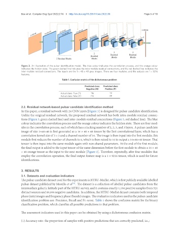
Figure 3. An illustration of the pulsar identification model. The blue colour indicates the convolution process, and the orange colour
indicates the hidden state. The green dashed line indicates the intra-module residual connections, and the red dashed line indicates the
inter-module residual connections. The inputs are the 1 × 48 × 48 grey images. There are four modules, and the outputs are 1 × 9216
features.

Table 1. Confusion matrix of the dichotomous problem

Predicted class: Predicted class:
Negative (N) Positive (P)
Actual class: True (T) TN TP
Actual class: False (F) FN FP

2.2. Residual network-based pulsar candidate identification method
In this paper, a residual network with 24 CNN layers [Figure 3] is designed for pulsar candidate identification.
Unlike the original residual network, the proposed residual network has both intra-module residual connec-
tions (Figure 3, green dashed line) and inter-module residual connections (Figure 3, red dashed line). The blue
colour indicates the convolution process and the orange colour indicates the hidden state. There are four mod-
ules in the convolution process, each of which has a stacking number of 2, 2, 3, and 3 layers. A pulsar candidate
image of size 1×48×48 is first generated as a 16 × 48 × 48 tensor by the first convolutional layer, which has a
convolution kernel size of 3 × 3 and a channel number of 16. The image is then input into the first module; this
module first reduces the number of channels to 8, which is then raised to 16 to output a 16×48×48 tensor. That
tensor is then input into the same module again with non-shared parameters. At the end of the first module,
the final output is added to the input tensor of the same dimension before the first module to obtain a 16 × 48
× 48 orange tensor as the input to the next module [Figure 3]. Therefore, repeatedly, after four modules that
employ the convolution operation, the final output feature map is a 1 × 9216 tensor, which is used for future
identifications.

3. RESULTS

3.1. Datasets and evaluation indicators
ThepulsarcandidatedatasetusedfortheexperimentsisHTRU-Medlat,whichisfirstpubliclyavailablelabelled
[6]
pulsar dataset published by Morello et al . The dataset is a collection of labelled pulsar candidates from the
intermediate galactic latitude part of the HTRU survey, and it contains exactly 1,196 positive samples from 521
distinctsourcesand89,996negativecandidates. Inaddition, theHTRU-Medlatdatasetcontainsbothtemporal
phase(ints)imagesandfrequencyphase(bands)images. Theevaluationindicatorsusedinthepulsarcandidate
identification problem are: Precision, Recall and F1-score. Table 1 shows the confusion matrix for the binary
classification problem, which classifies all possible predictions in that problem.

The assessment indicators used in this paper can be obtained by using a dichotomous confusion matrix.

(1) Accuracy rate: the proportion of samples with positive predictions that are correctly predicted, i.e.,: