Page 41 - Read Online

Fabbrini et al. Microbiome Res Rep 2023;2:25 https://dx.doi.org/10.20517/mrr.2023.25 Page 11 of 18

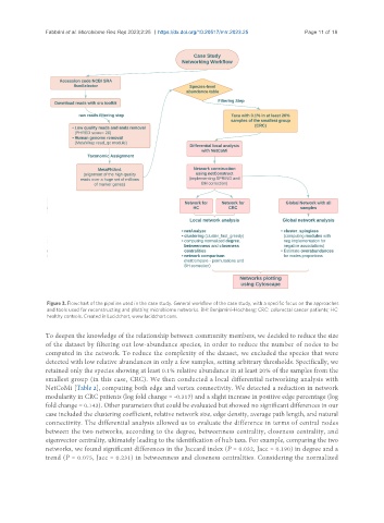
Figure 3. Flowchart of the pipeline used in the case study. General workflow of the case study, with a specific focus on the approaches
and tools used for reconstructing and plotting microbiome networks. BH: Benjamini-Hochberg; CRC: colorectal cancer patients; HC:
healthy controls. Created in Lucidchart, www.lucidchart.com.

To deepen the knowledge of the relationship between community members, we decided to reduce the size
of the dataset by filtering out low-abundance species, in order to reduce the number of nodes to be
computed in the network. To reduce the complexity of the dataset, we excluded the species that were
detected with low relative abundances in only a few samples, setting arbitrary thresholds. Specifically, we
retained only the species showing at least 0.1% relative abundance in at least 20% of the samples from the
smallest group (in this case, CRC). We then conducted a local differential networking analysis with
NetCoMi [Table 2], computing both edge and vertex connectivity. We detected a reduction in network
modularity in CRC patients (log fold change = -0.317) and a slight increase in positive edge percentage (log
fold change = 0.143). Other parameters that could be evaluated but showed no significant differences in our
case included the clustering coefficient, relative network size, edge density, average path length, and natural
connectivity. The differential analysis allowed us to evaluate the difference in terms of central nodes
between the two networks, according to the degree, betweenness centrality, closeness centrality, and
eigenvector centrality, ultimately leading to the identification of hub taxa. For example, comparing the two
networks, we found significant differences in the Jaccard index (P = 0.032, Jacc = 0.190) in degree and a
trend (P = 0.075, Jacc = 0.231) in betweenness and closeness centralities. Considering the normalized