Page 28 - Read Online

Xu et al. J Surveill Secur Saf 2020;1:16-33 I http://dx.doi.org/10.20517/jsss.2020.04 Page 21

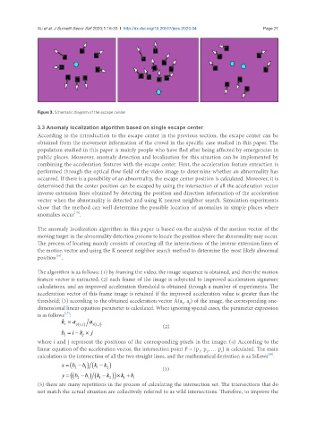
Figure 3. Schematic diagram of the escape center

3.3 Anomaly localization algorithm based on single escape center
According to the introduction to the escape center in the previous section, the escape center can be
obtained from the movement information of the crowd in the specific case studied in this paper. The
population studied in this paper is mainly people who have fled after being affected by emergencies in
public places. Moreover, anomaly detection and localization for this situation can be implemented by
combining the acceleration features with the escape center. First, the acceleration feature extraction is
performed through the optical flow field of the video image to determine whether an abnormality has
occurred. If there is a possibility of an abnormality, the escape center position is calculated. Moreover, it is
determined that the center position can be escaped by using the intersection of all the acceleration vector
inverse extension lines obtained by detecting the position and direction information of the acceleration
vector when the abnormality is detected and using K nearest neighbor search. Simulation experiments
show that the method can well determine the possible location of anomalies in simple places where
[15]
anomalies occur .

The anomaly localization algorithm in this paper is based on the analysis of the motion vector of the
moving target in the abnormality detection process to locate the position where the abnormality may occur.
The process of locating mainly consists of counting all the intersections of the inverse extension lines of
the motion vector and using the K nearest neighbor search method to determine the most likely abnormal
[16]
position .

The algorithm is as follows: (1) by framing the video, the image sequence is obtained, and then the motion
feature vector is extracted; (2) each frame of the image is subjected to improved acceleration signature
calculations, and an improved acceleration threshold is obtained through a number of experiments. The
acceleration vector of this frame image is retained if the improved acceleration value is greater than the
threshold; (3) according to the obtained acceleration vector A(a , a ) of the image, the corresponding one-
y
x
dimensional linear equation parameter is calculated. When ignoring special cases, the parameter expression
[17]
is as follows :
k = a a
l y ( ) x ( ) (2)
, ij
, ij
b = l ik− l × j
where i and j represent the positions of the corresponding pixels in the image; (4) According to the
linear equation of the acceleration vector, the intersection point P = {p , p , … p } is calculated. The main
s
2
1
calculation is the intersection of all the two straight lines, and the mathematical derivation is as follows :
[18]
x = (b − b ) (k − k )
2 1 1 2 (3)
y = ( ( b − 2 b 1 ) (k − 1 k 2 )) k× 1 + b 1
(5) there are many repetitions in the process of calculating the intersection set. The intersections that do
not match the actual situation are collectively referred to as wild intersections. Therefore, to improve the