Page 82 - Read Online

Page 6 of 31 Shu et al. J. Mater. Inf. 2025, 5, 36 https://dx.doi.org/10.20517/jmi.2025.13

usually no one universal best ML algorithm for materials research. The selection of an appropriate model
based on the available data and the prior knowledge and assumptions related to the specific research
problem. Each algorithm has its advantages and is suitable for different types of problems. It is critical to
select the appropriate model based on the specific characteristics of the dataset and the problem. This
requires a comprehensive understanding of material properties and their relationship to system variables
and parameters [73-75] . ML can be divided into supervised, unsupervised, semi-supervised, and reinforcement
learning [76,77] . Among these, supervised learning is the most widely applied method in ML. Its primary goal is
to predict new input data by learning the mapping relationship between input features and known target
variables. Supervised learning tasks can be divided into two main categories: regression and classification .
[78]
Additionally, ML models can be divided into three major categories based on their complexity and
structure: shallow learning models, ensemble learning models, and deep learning models.

Shallow learning models
Shallow learning models are relatively simple ML algorithms typically used when the data is simple, and the
relationships between features and target variables are linear or uncomplicated. Compared to more complex
models such as deep learning networks, shallow learning models are computationally less expensive and
easier to interpret, making them particularly useful when dealing with small datasets or when model
interpretability is crucial. Linear regression is a common shallow learning model that predicts continuous
values based on the assumption of a linear relationship between input features and the target variable. The
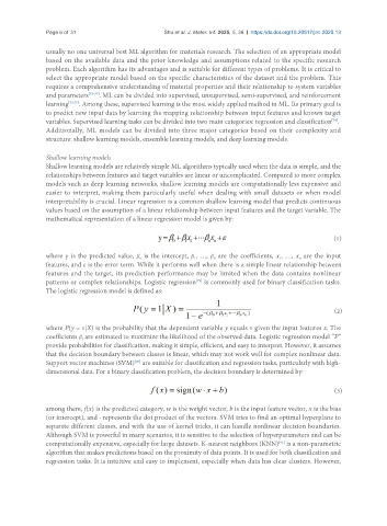
mathematical representation of a linear regression model is given by:

(1)

where y is the predicted value, β is the intercept, β , …, β are the coefficients, x , …, x are the input
n
n
1
1
0
features, and ε is the error term. While it performs well when there is a simple linear relationship between
features and the target, its prediction performance may be limited when the data contains nonlinear
[79]
patterns or complex relationships. Logistic regression is commonly used for binary classification tasks.
The logistic regression model is defined as:
(2)

where P(y = 1|X) is the probability that the dependent variable y equals 1 given the input features x. The
coefficients β are estimated to maximize the likelihood of the observed data. Logistic regression model “P”
i
provide probabilities for classification, making it simple, efficient, and easy to interpret. However, it assumes
that the decision boundary between classes is linear, which may not work well for complex nonlinear data.
Support vector machines (SVM) are suitable for classification and regression tasks, particularly with high-
[80]
dimensional data. For a binary classification problem, the decision boundary is determined by:

(3)

among them, f(x) is the predicted category, w is the weight vector, b is the input feature vector, x is the bias
(or intercept), and · represents the dot product of the vectors. SVM tries to find an optimal hyperplane to
separate different classes, and with the use of kernel tricks, it can handle nonlinear decision boundaries.
Although SVM is powerful in many scenarios, it is sensitive to the selection of hyperparameters and can be
computationally expensive, especially for large datasets. K-nearest neighbors (KNN) is a non-parametric
[81]
algorithm that makes predictions based on the proximity of data points. It is used for both classification and
regression tasks. It is intuitive and easy to implement, especially when data has clear clusters. However,