Page 40 - Read Online

Chen et al. J Mater Inf 2022;2:19 https://dx.doi.org/10.20517/jmi.2022.23 Page 13 of 21

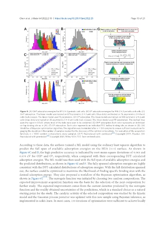
Figure 9. (A) OH* adsorption energies for 871 2 × 2 periodic unit cells. (B) O* adsorption energies for 998 2 × 2 periodic unit cells. (C)
OH* adsorption. The linear model was trained on 871 symmetric 2 × 2 unit cells (blue dots) and tested on 76 asymmetric 3 × 4 unit
cells (red crosses). The linear model used 15 parameters. (D) O* adsorption. The linear model was trained on 998 symmetric 2 × 2 unit
cells (blue dots) and tested on 36 asymmetric 3 × 4 unit cells (red crosses). The linear model used 55 parameters. The dashed lines
span the region ± 0.1 eV, where most of the data were seen to be contained. (E) OH* adsorption. Each color represents an individual
on-top binding site as in (A). (F) O* adsorption. Each color represents an individual FCC hollow binding site, as shown in (B). (G)
Workflow of Bayesian optimization algorithm. The algorithm was terminated after n = 150 samples to ensure sufficient evaluations for
gauging the deviation in the number of samples needed for the discovery of the optimal compositions. For evaluation of the acquisition
function, n = 1000 random compositions were sampled. (A-F) Reproduced with permission [60] . Copyright 2019, Elsevier. (G)
Reproduced with permission [84] . Copyright 2021, Wiley-VCH. FCC: face-centered cubic.

According to these data, the authors trained a ML model using the ordinary least squares algorithm to
predict the full span of available adsorption energies on the HEA (111) surface. As shown in
Figure 9C and D, the high predictive accuracy is indicated by root-mean-square deviations of 0.063 and
0.076 eV for OH* and O*, respectively, when compared with their corresponding DFT calculated
adsorption energies. The ML model was then used with the full span of available adsorption energies and
the predicted distributions, as shown in Figure 9E and F. The fully spanned adsorption energies are highly
consistent with the DFT-calculated distributions of adsorption energies. With the full distribution spanned
out, the surface could be optimized to maximize the likelihood of finding specific binding sites with the
desired adsorption energy. They also proposed a workflow of the Bayesian optimization algorithm, as
shown in Figure 9G [80,84] . The surrogate function was initiated by choosing two random compositions. The
expected improvement acquisition function was the basis for the selection of the next composition for
further study. The expected improvement comes from the current densities predicted by the surrogate
function and the readily obtained uncertainties of the predictions, which is a standard choice as a natural
starting point for the study. The catalytic activity of the selected composition was studied by the kinetic
model and the Gaussian process posterior was updated with this new sample using Bayesian inference, as
implemented in scikit-learn. In most cases, 150 iterations of optimization were sufficient to achieve locally