Page 72 - Read Online

Page 265 Su et al. Intell Robot 2022;2(3):244­74 I http://dx.doi.org/10.20517/ir.2022.17

the back-door path and front-door path are first introduced, which are helpful for the understanding of the
front-door criterion. A causal path connecting and which begins with an arrow leading to is called a
back-door path (e.g., ← ... ), while a path starting with an arrow pointing away from is called a front-door
path (e.g., → ... ). If the front-door criterion is satisfied, there exits a mediator variable such that: (i)
there are no backdoor paths from to ; and (ii) all backdoor paths from to are blocked by . Formally,
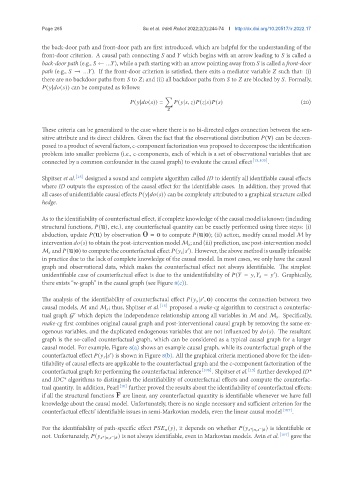
( | ( )) can be computed as follows:
∑
( | ( )) = ( | , ) ( | ) ( ) (20)

These criteria can be generalized to the case where there is no bi-directed edges connection between the sen-
sitive attribute and its direct children. Given the fact that the observational distribution (v) can be decom-
posed to a product of several factors, c-component factorization was proposed to decompose the identification
problem into smaller problems (i.e., c-components, each of which is a set of observational variables that are
connected by a common confounder in the causal graph) to evaluate the causal effect [15,105] .

Shpitser et al. [15] designed a sound and complete algorithm called ID to identify all identifiable causal effects
where ID outputs the expression of the causal effect for the identifiable cases. In addition, they proved that
all cases of unidentifiable causal effects ( | ( )) can be completely attributed to a graphical structure called
hedge.

As to the identifiability of counterfactual effect, if complete knowledge of the causal model is known (including
structural functions, (u), etc.), any counterfactual quantity can be exactly performed using three steps: (i)
abduction, update (u) by observation O = o to compute (u|o); (ii) action, modify causal model M by
intervention ( ) toobtainthepost-interventionmodel M ; and(iii)prediction,usepost-interventionmodel
M and (u|o) tocomputethecounterfactualeffect ( | ). However, theabovemethodisusuallyinfeasible
′
in practice due to the lack of complete knowledge of the causal model. In most cases, we only have the causal
graph and observational data, which makes the counterfactual effect not always identifiable. The simplest
unidentifiable case of counterfactual effect is due to the unidentifiability of ( = , = ). Graphically,
′
there exists “w-graph” in the causal graph (see Figure 8(c)).

The analysis of the identifiability of counterfactual effect ( | ,o) concerns the connection between two
′
causal models, M and M ; thus, Shpitser et al. [15] proposed a make-cg algorithm to construct a counterfac-
tual graph G which depicts the independence relationship among all variables in M and M . Specifically,
′
make-cg first combines original causal graph and post-interventional causal graph by removing the same ex-
ogenous variables, and the duplicated endogenous variables that are not influenced by ( ). The resultant
graph is the so-called counterfactual graph, which can be considered as a typical causal graph for a larger
causal model. For example, Figure 8(a) shows an example causal graph, while its counterfactual graph of the
counterfactual effect ( | ) is shown in Figure 8(b). All the graphical criteria mentioned above for the iden-
′
tifiability of causal effects are applicable to the counterfactual graph and the c-component factorization of the
counterfactual graph for performing the counterfactual inference [106] . Shpitser et al. [15] further developed ID*
and IDC* algorithms to distinguish the identifiability of counterfactual effects and compute the counterfac-
tual quantity. In addition, Pearl [10] further proved the results about the identifiability of counterfactual effects:
if all the structural functions F are linear, any counterfactual quantity is identifiable whenever we have full
knowledge about the causal model. Unfortunately, there is no single necessary and sufficient criterion for the
counterfactual effects’ identifiable issues in semi-Markovian models, even the linear causal model [107] .

For the identifiability of path-specific effect ( ), it depends on whether ( | , | ¯ ) is identifiable or
+
−
not. Unfortunately, ( | , | ¯ ) is not always identifiable, even in Markovian models. Avin et al. [107] gave the
−
+