Page 70 - Read Online

Page 263 Su et al. Intell Robot 2022;2(3):244­74 I http://dx.doi.org/10.20517/ir.2022.17

U C

U S U Y U S C U Y

S Y S Y

(a) A Simple causal graph (b) A Simple causal graph
with no confounder between with an observational
sensitive attribute and confounder between sensitive
outcome. attribute and outcome.

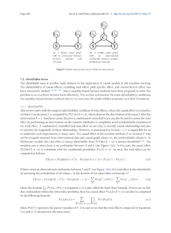
Figure 7. Simple causal graphs under Markovian assumption.

7.2. Identifiable issue
The identifiable issue is another main obstacle to the application of causal models in fair machine learning.
The identifiability of causal effects, including total effect, path-specific effect, and counterfactual effect, has
been extensively studied [10,100–103] . Many causality-based fairness methods have been proposed to solve this
problem so as to achieve fairness more effectively. This section summarizes the main identifiability conditions,
the causality-based fairness methods that try to overcome the unidentifiable situations, and their limitations.

7.2.1. Identifiability
This review starts with the simplest identifiability condition of total effects, where the causal effect of a sensitive
attribute on decision is computed by ( | ( = )), which denotes the distribution of decision after the
intervention = . Similar to causal discovery, randomized controlled trials can also be used to assess the total
effect by performing an intervention on the sensitive attributes to completely avoid unidentifiable situations of
the total effect. A randomized controlled trial may allow us not only to identify causal relationships but also
to estimate the magnitude of these relationships. However, as mentioned in Section 7.1, it is impossible for us
to undertake such experiments in many cases. The causal effect of the sensitive attribute on decision may
not be uniquely assessed from observational data and causal graph alone, i.e., the unidentifiable situation. In
Markovian models, the total effect is always identifiable, since ( | ( = )) is always identifiable [10] . The
simplest case is when there is no confounder between and (see Figure 7(a)). In this case, the causal effect
( | ( = )) is consistent with the conditional probability ( | = ). As such, the total effect can be
computed as follows:
+ − + − (15)
( ) = ( | ( = )) − ( | ( = )) = ( | ) − ( | )

Ifthere exists an observational confounder between and (see Figure 7(b)), the total effect is also identifiable
by summing the probabilities of all values in the domain of the observable confounder :
∑ ∑
+
+
−
−
( ) = ( | ( = )) − ( | ( = )) = ( | , ) ( ) − ( | , ) ( ) (16)

where the formula ∑ ( | , ) ( ) in Equation (16) is also called the back-door formula. If there are no hid-
den confounders within the observable attributes, then the causal effect ( | ( = )) can also be computed
by the following formula:
∑ ∏
( | ( )) = ( | ( )) (17)
V\{ , }, = ∈V\{ }
where ( ) represents the parent variables of . It is easy to see that the total effects computed by Equations
(16) and (17) can produce the same result.