Page 76 - Read Online

Lv et al. Intell Robot 2022;2(2):168­79 I http://dx.doi.org/10.20517/ir.2022.09 Page 174

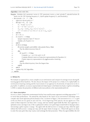
Algorithm 1 SAC with TRC.
Require: Initialize SAC parameter vector , CPC parameter vector , total episode , episode horizon ,
batch size , CPC training frequency , labels update frequency , and threshold .
1: for episode = 0 . . . − 1 do
2: opponent choose policy −1
3: for step = 0 . . . − 1 do
( 1 1 −1 )
1
4: ∼ | ,

1
5: −1 ∼ −1 ( −1 | , −1 )

(
1
−1
1
6: 1 , −1 ∼ 1 , −1 , | , , , −1 )
+1 +1 +1 +1
1
1
−1
−1
1
−1
1
7: ← ∪ {( , , , ( , , , ), 1 +1 , −1 )}

+1
8: end for
9: ← ∪
10: if mod == 0 then
11: Sample trajectory batch T from
12: Update by Equation (5)
13: end if
14: if | | == then
15: if random sample a probability value greater than then
16: Pop the oldest trajectory from
17: else
18: if mod == 0 then
19: Compute : = ( ) for each in
20: Compute distance matrix of trajectory representations by Equation (6)
21: Cluster trajectory representations by agglomerative clustering
22: end if
23: Pop the oldest trajectory from the largest class
24: end if
25: end if
26: Update by SAC algorithm.
27: end for
4. RESULTS
We evaluate our approach in a more complex soccer environment and compare the average returns during RL
training against three baselines. We also discuss the impact of the proportion of data in the replay buffer on
reinforcement learning training and the improvement of our approach to the diversity of trajectories in the re-
play buffer. In addition, we analyze representational clustering by t-distributed stochastic neighbor embedding
(t-SNE) to analyze the properties of different adversary policies at the representational level.
4.1. Game description
Soccer is a classic competitive environment that has been used by many opponent modeling approaches [11,13]
to verify their performance. We extend the rules based on the classic soccer environment and design more
complex rule-based opponent policies based on this. As shown in Figure 2, the environment is a 15 × 15 grid
world, and there are two goals on each end line. At the beginning of the episode, the two agents are in the
center of their respective end lines with 0 energy, and one random agent holds the ball. Each agent has 13
optional actions, moving to any of the 12 grid points within a two-grid range around itself or staying in place,
but moving 2 grids requires 2 energy. The agent with the ball recovers 0.5 energy per step, while the agent
without the ball recovers 1 energy per step, and the upper limit of energy is 2. When both agents are about
to enter the same grid, they stop in place and exchange the ball possession. When the agent dribbles the ball