Page 40 - Read Online

Liu et al. Intell Robot 2024;4(4):503-23 I http://dx.doi.org/10.20517/ir.2024.29 Page 509

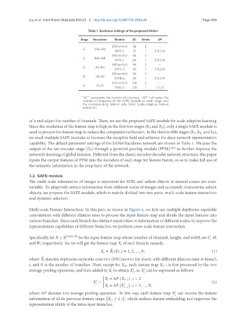
Table 1. Backbone settings of the proposed SANet

Stage Resolution Module #C Stride #P
DSConv3×3 32 2 -
336×336
E 1
SAFE×1 32 1 3 (1,2,4)
DSConv3×3 64 2 -
168×168
E 2
SAFE×1 64 1 3 (1,2,4)
DSConv3×3 96 2 -
84×84
E 3
SAFE×3 96 1 3 (1,2,4)
DSConv3×3 96 2 -
42×42
E 4
SAFE×6 96 1 3 (1,2,4)
DSConv3×3 128 2 -
21×21
E 5
SAFE×3 128 1 2 (1,2)
“#C” represents the number of channels. “#P” indi-cates the
number of branches of the SAFE module at each stage and
the corresponding dilation rate. SAFE: Scale-adaptive feature
extraction.
of 2 and adjust the number of channels. Then, we use the proposed SAFE module for scale-adaptive learning.
Since the resolution of the feature map is high in the first two stages (E 1 and E 2), only a single SAFE module is
used toprocessthefeaturemap toreducethecomputationalburden. In thethird tofifth stages(E 3, E 4, andE 5),
we stack multiple SAFE modules to increase the receptive field and enhance the deep network representation
capability. The default parameter settings of the SANet backbone network are shown in Table 1. We pass the
output of the last encoder stage (E 5) through a pyramid pooling module (PPM) [44] to further improve the
network’s learning of global features. Different from the classic encoder-decoder network structure, this paper
inputs the output features of PPM into the decoders of each stage for feature fusion, so as to make full use of
the semantic information in the deep layer of the network.

3.2. SAFE module
The multi-scale information of images is important for SOD, and salient objects in natural scenes are scale-
variable. To adaptively extract information from different scales of images and accurately characterize salient
objects, we propose the SAFE module, which is mainly divided into two parts: multi-scale feature interaction
and dynamic selection.

Multi-scale Feature Interaction: In this part, as shown in Figure 4, we first use multiple depthwise separable
convolutions with different dilation rates to process the input feature map and divide the input features into
various branches. Since each branch has distinct sensitivities to information of different scales, to improve the
representation capabilities of different branches, we perform cross-scale feature interaction.

Specifically, let ∈ R × × be the input feature map whose number of channels, height, and width are , ,
and , respectively. So, we will get the feature map of each branch, namely,

= $ ( ), = 1, 2, ..., , (1)
where $ denotes depthwise separable conv3×3 (DSConv3×3 for short) with different dilation rates at branch
, and is the number of branches. Next, except for , each feature map −1 is first processed by the 3×3
average pooling operation, and then added to to obtain , so can be expressed as follows:
′
′

(
+ ( −1 ) , = 2
′
= (2)

+ ′ , = 3, ..., ,
−1
where denotes 3×3 average pooling operation. In this way, each feature map can receive the feature
′

information of all its previous feature maps , ⩽ , which realizes feature embedding and improves the
representation ability of the intra-layer branches.