Page 25 - Read Online

Ji et al. Intell Robot 2021;1(2):151-75 https://dx.doi.org/10.20517/ir.2021.14 Page 169

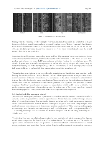
Figure 10. Sample patterns of different classes.

training while the remaining 10% for testing for every class. In anomaly detection, the distribution of images
is comprised of 57% normal images and 43% images with various types of defects. In anomaly classification,
there are ten classes in total that are to be classified; their distributions are: 57%, 7%, 2%, 4%, 1%, 1%, 7%, 2%,
17%, and 2%. Input greyscale images were resized to 186 × 256 pixels before being fed into the neural
network for training and prediction.

Four convolutional layers, two max-pooling layers, and four fully connected layers were connected for the
deep convolutional neural network, and the convolutional kernel size was set as 3 × 3 pixels. We used max-
pooling units of size 2 × 2 pixels. ReLU was used as an activation function for convolutional layers. We
added a dropout layer as an effective regularization method after max-pooling to reduce overfitting by
randomly dropping out nodes during training. After the convolutional and max-pooling layers, we used
fully connected layers to perform high-level reasoning in a convolution neural network.

We ran the deep convolutional neural network model for detection and classification tasks separately while
keeping the training and testing images the same and only adjusting the number of output classes for the
network classifiers at the end of the network. The learning rate of the Adam optimizer was set as 0.001 for
training the model. For both the binary classification of detection tasks and the multi-class classification of
classification tasks, we counted the number of true positives, true negatives, false positives, and false
negatives. The binary classification accuracy was calculated as 87.45% and F1-score as 88.33%. The
performance is acceptable and substantially improves the performance of the existing auto-detect method
based on image process techniques and man-made feature representations in operation.

5.4. Application 2: Siamese neural network
We conducted training and prediction experiments for classification tasks with four classes of data which
comprise normal images and three common types of defects. We used an equal number of images for each
class. We created the training data samples for Siamese neural network, which is much easier than the
classic convolutional neural network datasets that require images to be labeled. Image samples were
randomly chosen from this dataset to form anchor-positive-negative trios. While sampling an image pair,
the two images were chosen from the same category with a probability of 0.5 with a corresponding label of y
= 0. Similarly, the images were chosen from two different categories with the remaining probability of 0.5
with the label y = 1.

Two identical four-layer convolutional neural networks were used to form the twin structure of the Siamese
neural network to perform the identification of rail surface defects. The batch size was 128. The number of
epochs was 50. The number of steps per epoch was 5. ReLU was used as an activation function. The neural
network optimizer used was Adam. During testing, data of matching pairs and non-matching pairs were