Page 88 - Read Online

Page 10 of 23 Li et al. J. Mater. Inf. 2025, 5, 43 https://dx.doi.org/10.20517/jmi.2025.17

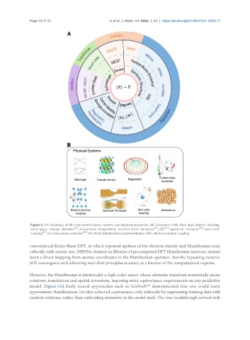
Figure 4. (A) Summary of ML-Ham architectures, models, and physical properties; (B) Examples of ML-Ham applications, including
band gaps, charge densities [61] , noncolinear magnetism, excited-state dynamics [62] , EPC [63] , quantum transport [64] , spin-orbit
coupling [65] and amorphous materials [66] . ML-Ham: Machine learning Hamiltonian; EPC: electron-phonon coupling.

conventional Kohn-Sham DFT, in which repeated updates of the electron density and Hamiltonian scale
cubically with system size. DHNNs, trained on libraries of precomputed DFT Hamiltonian matrices, instead
learn a direct mapping from atomic coordinates to the Hamiltonian operator, thereby bypassing iterative
SCF convergence and delivering near–first-principles accuracy at a fraction of the computational expense.

However, the Hamiltonian is intrinsically a high-order tensor whose elements transform nontrivially under
rotations, translations and spatial inversions, imposing strict equivariance requirements on any predictive
[68]
model [Figure 5A]. Early neural approaches such as SchNorb demonstrated that one could learn
approximate Hamiltonians, but they achieved equivariance only indirectly by augmenting training data with
random rotations, rather than embedding symmetry in the model itself. The true breakthrough arrived with