Page 87 - Read Online

Page 81 Bah et al. Intell Robot 2022;2(1):72­88 I http://dx.doi.org/10.20517/ir.2021.16

2.4. Training phase
In this work, the models were trained on google colab pro with GPU availability, and they were implemented
using Keras2 and Python3. The training was conducted in two phases. We trained the network with a deep
Convolutional Neural Network without Residual Blocks in the first phase. Then after noticing that the accu-
racy is not increasing that much, we added a residual block to help the network generalize well and improve
the success rate. The two models were allowed to train for 100 epochs with a batch size of 64. The optimizer
used to train the models is the Nadam [39] based on the stochastic gradient descent algorithm, with a learning
rate of 0.001, beta_1 parameter value of 0.9, beta_2 is 0.999. and the loss function used is the categorical cross-
entropy [40] function since we have a model with more than two outputs. For this work, having a problem of
imbalance data, we highly weighted the classes with few number of samples and gave small weights to those
with big number of samples. The learning rate is regulated during the training by the callback class ReduceL-
ROnPlateau [41] implemented in the Keras library. This class has the particularity to update the learning to the
minimum value (min_lr = 0.0000001) when there is no improvement of the validation accuracy and will stop
the training after 15 epochs. We chose 15 epochs to allow the training to last for a long time. Another callback
class used is the EarlyStopping [42] . The patience here is set to 30, and finally, we used the ModelCheckpoint
to save the model after each improvement of the validation accuracy.

3. RESULTS
ThetrainingprocessofthetwomodelsrespectivelythebasicCNNandResNetbasedCNNonFERGITdataset,
and the ResNet based CNN on CK+ dataset took only 119 minutes of total training time with colab pro (K80
GPUs, 25GB RAM).

3.1. Performance Analysis
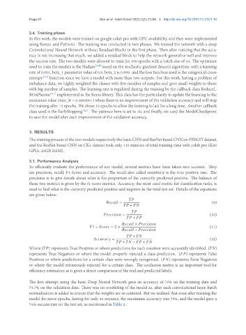
To efficiently evaluate the performance of our model, several metrics have been taken into account. They
are precision, recall, F1-Score and accuracy. The recall also called sensitivity is the true positive rate. The
precision is to give details about what is the proportion of the correctly predicted positive. The balance of
these two metrics is given by the f1-score metrics. Accuracy, the most used metric for classification tasks, is
used to find what is the correctly predicted positive and negative in the total test set. Details of the equations
are given below:

= (9)
+

= (10)
+
×
1 − = 2 × (11)
+
+
= (12)
+ + +
Where ( ) represents True Positives or where predictions for each emotion were accurately identified. ( )
represents True Negatives or where the model properly rejected a class prediction. ( ) represents False
Positives or where predictions for a certain class were wrongly recognized. ( ) represents False Negatives
or where the model erroneously rejected for a certain class. The confusion matrix is an important tool for
efficiency estimation as it gives a direct comparison of the real and predicted labels.

The first attempt using the basic Deep Neural Network gave an accuracy of 75% on the training data and
73.7% on the validation data. There was no overfitting of the model as, after each convolutional layer, batch
normalization is added to ensure that the weights are re-centered. But we realized that even after training the
model for more epochs, lasting for only 44 minutes, the maximum accuracy was 75%, and the model gave a
74% success rate on the test set, as mentioned in Table 2.