Page 33 - Read Online

Page 260 Sun et al. Intell Robot 2023;3(3):257-73 I http://dx.doi.org/10.20517/ir.2023.17

Table 1. Physical meanings in path following control
Parameter Physical meaning
the mass of vehicle
the lateral forces of the front tire

the lateral forces of the rear tire

the tire slip angle of the front tire

the tire slip angle of the rear tire

the vehicle sideslip angle
the yaw inertia of the vehicle

the center of gravity of the vehicle to the front wheel axis

the center of gravity of the vehicle to the rear wheel axis

the front tire cornering stiffness

the rear tire cornering stiffness

the lateral offset from the vehicle center of gravity to the
closest on the desired path
the error between the actual heading angle ℎ and the
desired heading angle
the yaw rare of the vehicle with ¤ ℎ =
the longitudinal velocity of the vehicle

the lateral velocity of the vehicle

the front-wheel steering angle

the curvilinear coordinate of point along the path from
an initial position predefined
the curvature of the desired path at the point .
( )
&$1 %86
3DWK SODQQLQJ 6WDWH VHQVLWLYH
(&8 (YHQW WULJJHU
7RUTXH
VHQVRU
6WHHULQJ
VKDIW
5HGXFHU
&XUUHQW 6WHHULQJ JHDU
0RWRU &OXWK
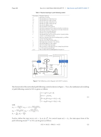
Figure 1. Path following control diagram with SS-ETC scheme.

TheframeworkofthenetworkedpathfollowingcontrolisshowninFigure1. Then,themathematicalmodeling
of path following control of AVs is given as follows


 ¤ = + + 1



 
 ¤ = − ( )
(1)
 ¤
 = 11 + 12 + 1 + 2



 ¤ = 21 + 22 + 2 + 3 .

with
( + ) ( − )
11 = − , 12 = −(1 + ),
2

2 2

( − ) ( + )
21 = , 22 = −( ),

1 = , 2 = .

Further, define the state vector ( ) = [ , , , ] , the control input ( ) = , the state-space form of the

path following model [32] of AVs can be given as follows
¤ ( ) = ( ) + ( ) + ( ) (2)