Page 89 - Read Online

Page 98 Zhou et al. Intell Robot 2023;3(1):95-112 I http://dx.doi.org/10.20517/ir.2023.05

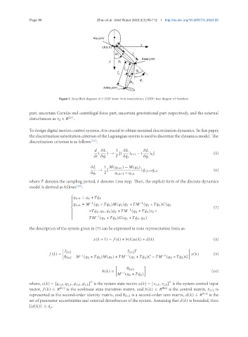
Figure 1. Simplified diagram of 2-DOF lower limb exoskeleton. 2-DOF: two-degree-of-freedom.

part, uncertain Coriolis and centrifugal force part, uncertain gravitational part respectively, and the external
disturbances as ∈ 2×1 .

To design digital motion control systems, it is crucial to obtain nominal discretization dynamics. In this paper,
thediscretizationsubstitutioncriterionoftheLagrangiansystemis used todiscretizethedynamicsmodel. The
discretization criterion is as follows [24] :
1
( ) → [( ) +1 − ( ) ] (5)
¤ ¤ ¤

1 ( +1 ) − ( )

→ [ ] ¤ , +1 ¤ , (6)
2 , +1 − ,
where denotes the sampling period, denotes time step. Then, the explicit form of the discrete dynamics
model is derived as follows [25] :


 +1 = + ¤




  ¤ +1 =
 −1 ( + ¤ ) ( ) ¤ + −1 ( + ¤ ) (
(7)

 + ¤ , , ¤ ) ¤ + −1 ( + ¤ ) −



 −1

 ( + ¤ ) ( + ¤ , )

the description of the system given in (7) can be expressed in state representation form as:
( + 1) = ( ) + ( ) ( ) + ( ) (8)

2×2 2×2
( ) = −1 −1 −1 ( ) (9)

0 2×2 ( + ¤ ) ( ) + ( + ¤ ) − ( + ¤ )

0 2×2
( ) = −1 (10)

( + ¤ )

where, ( ) = [ 1, , 2, , ¤ 1, , ¤ 2, ] is the system state vector, ( ) = [ 1, , 2, ] is the system control input

vector, ( ) ∈ 4×1 is the nonlinear state transition matrix, and ( ) ∈ 4×2 is the control matrix, 2×2 is
represented as the second-order identity matrix, and 0 2×2 is a second-order zero matrix, ( ) ∈ 4×1 is the
set of parameter uncertainties and external disturbances of the system. Assuming that ( ) is bounded, then
|| ( )|| ≤ .