Page 7 - Read Online

Ma et al. Complex Eng Syst 2023;3:10 I http://dx.doi.org/10.20517/ces.2023.14 Page 3 of 14

2.1. Preliminaries

Lemma 1 [18] Consider the following system as

¤ = ( ), (0) = 0, ∈ R (1)

If there exists a positive definite Lyapunov function ( ), which satisfies ( ) ≤ − 1 ( ) − 1 ( ) + , where
¤
1 , 1, and are all positive constants. 0 < < 1, > 1 are real numbers. Then the origin of the system (2) is
1 1
fixed-time stable, and the settling time is bounded by 1 ≤ + with 0 < < 1.
1 (1− ) 1 ( −1)
Lemma 2 [16] The Gaussian error function is defined as follows:
¹
2 −2 2
erf( ) = √ dt (2)
0
where is the natural constant. If 0 ≤ < 1, then the Gaussian error function will satisfy ≤ erf( ) ≤ 2 .
1
2

Lemma 3 [19] For ∈ R and > 0, one gets the following chain of inequalities: tanh( ) < erf( ) < | |.

Lemma 4 [20] The following inequality will hold | | − ≤ tanh( ) for any > 0 and for any ∈ R, where
= −( +1) . Then, = 0.2785 can be obtained.
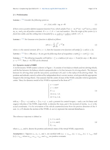
2.2. Dynamic model of WMR
A nonholonomic WMR system is shown in Figure 1. It consists of two balance wheels and two driving wheels,
and the line between the balance wheels is perpendicular to the line between the driving wheels. The distance
between the driving wheel and the barycentric coordinate is , and is the radius of the driving wheel. The
position and attitude control is achieved by independent direct current motors, which provide the appropriate
torques to the driving wheels. One assumes that the center of mass of the WMR coincides with the geometric
center. Then, the dynamic model of the WMR is expressed in the form of [21]

 ¤ = cos





 ¤ = sin



= (3)
¤



 ¤ = 1 + 1




 ¤ = 2 + 2

1
with 1 = ( 1 − 2 ), and 2 = ( 1 + 2 ). 1 and 2 present the control torques. and are the linear and

angular velocities of the WMR, respectively. denotes the mass, and the moment of inertia. ( , ) is the
actual coordinates. is the orientation of the vehicle counterclockwise from the positive direction of the
axis. ( ¤, ¤ , ) denotes the motion of the WMR. 1 and 2 represent the external disturbances.

¤
The reference trajectory is defined as
 ¤ = cos



¤ = sin (4)


 ¤
=

where , , and denote the position and attitude states of the virtual WMR, respectively.
, And
Assumption 1: Suppose , ¤ , , and ¤ are satisfied with | | ≤ max , | ¤ | ≤ 1 max , | | ≤ max
are positive constants.
|¤ | ≤ 1 max , where max , 1 max , max , and 1 max