Page 62 - Read Online

Page 48 Harib et al. Intell Robot 2022;2(1):37-71 https://dx.doi.org/10.20517/ir.2021.19

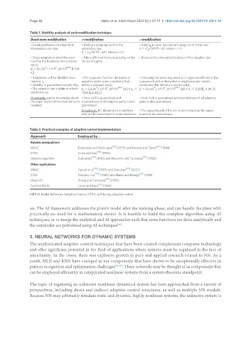
Table 1. Stability analysis of each modification technique
Dead-zone modification σ-modification ϵ-modification
• Developed based on adaptation • Adding a damping term to the • Adding an error dependent leakage term to the law:
T
hibernation principle. adaptation law: K = -Γ e BP(Ψ - ϵK), where ϵ > 0
T K
K = Γ (Ψe PB - σK), where σ > 0
K
• Stops adaptation when the error • Takes different forms depending on the • Reduces the unbounded behavior of the adaptive law
touches the boundary of a compact choice of sigma
set β :
d
T
n
β = {(e,ΔK ), e∈R , ΔK∈R N×m ||e|| ≤
d
e }
d
• Adaptation will be disabled once • The Lyapunov function derivative is • Following the same argument as in sigma modification: the
reaches e negative under some conditions that Lyapunov function derivative is negative under certain
d
• Stability is guaranteed outside of β define a compact set β : conditions that define a compact set β :
ϵ
d
σ
n
T
T
n
• The adaptive law is defined in both β = {(e,ΔK ), e∈R , ΔK∈R N×m ||e|| ≤ e ∧ β = {(e,ΔK ), e∈R , ΔK∈R N×m ||e|| ≤ e ∧ (||ΔK|| ≤ ΔK )}
σ σ ϵ ϵ F ϵ
conditions as: (||ΔK|| ≤ ΔK )}
σ
F
Drawbacks: a prior knowledge about • Error UUB is guaranteed and • Error UUB is guaranteed and boundedness of all adaptive
the upper bound of the disturbance is boundedness of all adaptive gains is also gains is also guaranteed
required guaranteed
Drawbacks: the damping term addition • The upper bound of the set is determined by the upper
may not be convenient in some situations bound of the disturbance
Table 2. Practical examples of adaptive control implementation
Approach Employed by…
Robotic manipulators
MRAC Dubowsky and DesForges [53] (1979) and Nicosia and Tomei [55] (1984)
[56]
STAC Koivo and Guo (1983)
Adaptive algorithm Dubowsky [54] (1981) and Horowitz and Tomizuka [57] (1986)
Other applications
MRAC Harrell et al. [49] (1987) and Davidson [47] (2021)
[48] [52]
STAC Davison et al. (1980) and Harris and Billings (1981)
Direct AC Zhang and Tomizuka [50] (1985)
[51]
Function Blocks Lukas and Kaya (1983)
MRACL Model Reference Adaptive Control; STAC: self-tuning adaptive control.
on. The AI framework addresses the plant’s model after the training phase, and can handle the plant with
practically no need for a mathematical model. It is feasible to build the complete algorithm using AI
techniques, or to merge the analytical and AI approaches such that some functions are done analytically and
the remainder are performed using AI techniques .
[62]
3. NEURAL NETWORKS FOR DYNAMIC SYSTEMS
The sophisticated adaptive control techniques that have been created complement computer technology
and offer significant potential in the field of applications where systems must be regulated in the face of
uncertainty. In the 1980s, there was explosive growth in pure and applied research related to NN. As a
result, MLN and RNN have emerged as key components that have shown to be exceptionally effective in
pattern recognition and optimization challenges [63-68] . These networks may be thought of as components that
can be employed efficiently in complicated nonlinear systems from a system-theoretic standpoint.

The topic of regulating an unknown nonlinear dynamical system has been approached from a variety of
perspectives, including direct and indirect adaptive control structures, as well as multiple NN models.
Because NN may arbitrarily simulate static and dynamic, highly nonlinear systems, the unknown system is